Introduction

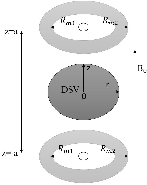
Conventional biplanar coils are used in open MRI scanners. Usually, two parallel discs that consist of symmetric and anti-symmetric coil patterns are used for transverse and longitudinal gradient coils, respectively. Recently, a three-channel cylindrical Z-gradient coil array was introduced [1]. In this work, we used the concept of coil arrays to design a two-channel bi-planar Z-gradient coil. The coil consists of two discs (Figure 1 ) which are divided into two sections along the radial direction where the current density of each section is written in terms of Fourier series expansions. The pattern of the coil windings for each section is determined from the stream function [2]. The radius of each section is varied until the most power-efficient design is obtained. The total dissipated DC power of the achieved two-channel design is compared to that of the conventional coil. Results showed that the power dissipated by the two-channel biplanar coil is less than the conventional Z-gradient coil by at least 25% for the specific coil dimensions used in this work while achieving the same gradient strength at the desired diameter of spherical volume (DSV).

Methods

As shown in Figure 1, channel one has the two first sections of upper and lower plates with radius $$$ R_{m1} $$$ while channel two has the rest of the sections i.e., the shaded annular regions in grey. The current density ($$$ J_{θi} $$$) of the two sections can be expanded as: $$$J_{\theta 1}(ρ)=\sum_{n=1}^{N}U_{n}\sin(nc(ρ-ρo))$$$, $$$R_{o} \leq ρ \leq R_{m1}$$$, $$$ρ_o=R_{o}$$$ and $$$J_{\theta 2}(ρ)=\sum_{n=1}^{N}U_{n}\sin(nc(ρ-ρo))$$$, $$$R_{m1} \leq ρ \leq R_{m2} $$$, $$$ρ_o=R_{m1}$$$, for section one and section two of the upper disc, respectively [3], where $$$c=\frac{\pi}{ρ_m-ρ_o}$$$ and $$$ρ_m$$$ is the maximum radius of the section [2]. The current density of the corresponding sections of the lower plate is equal in magnitude but opposite in direction to that of the upper disc. The gradient field is determined from the following Biotsavart’s formula for each section, i, $$$ B_z(x_o,y_o,z_o)=\frac{\mu_0}{4\pi}\int_{ρ_o}^{ρ_m}\int_{0}^{2\pi}\frac{J_{\theta i}(ρ-y_o\sin(⁡\theta)-x_o\cos(⁡\theta))}{{\big(\sqrt{(x_o- ρ\cos(⁡\theta))^2+(y_o-ρ \sin(⁡\theta))^2+(z_o-z)^2)}}\big)^{3}}ρ d\theta dρ $$$ . A set of linear equations are then formulated to achieve the target field at each 256 equally distributed points in the DSV [2]. We used N=5 Fourier series coefficients similar to previously published work [2]. Tikhonov’s regularization with penalty function (similar to [4]) was used to solve the set of linear equations and determine the unknown Fourier series coefficients ($$$U_{n}$$$). The regularization parameter (λ) in Tikhonov’s regularization was iteratively selected from a predetermined range to minimize the deviation from the target gradient field [5]. Using the calculated Fourier series coefficients ($$$U_n$$$), the stream function of each section was determined [2]. The winding pattern and the current of each channel are then obtained from the stream function. It is noted that the number of coil windings is iteratively determined to attain the least dissipated power for each $$$R_{m1}$$$. We used, $$$R_{o}=1cm$$$, $$$R_{m2} =40cm$$$, size of the DSV =$$$38cm$$$, gap between the two discs (2a) =$$$49cm$$$ (similar to [4]), target gradient field $$$=25 \frac{mT}{m}$$$ . $$$R_{m1}$$$ varies from 9 cm to 33 cm with a radial increment (ΔR) =3 cm to obtain the optimal size of the two sections that minimizes the dissipated power.

Results

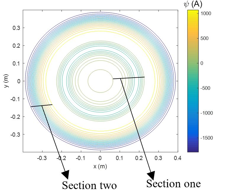
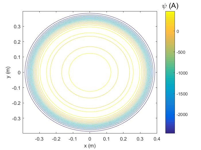
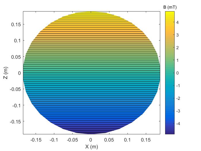
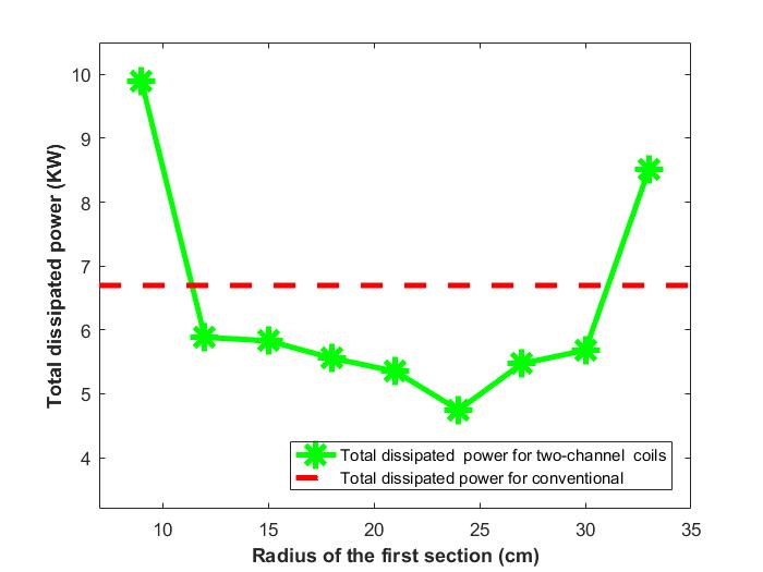
The optimization process resulted in 9 different designs for the two-channel coil from which the configuration that produced the least power dissipation was chosen. Figure 2 shows the winding patterns of each section of the best design for the upper disc. Channel one and channel two had a current of 92.7 A and 178.6 A, respectively. Using the same design process, we obtained a conventional coil design (Figure 3) driven by 225.9 A to achieve the same target field. It is noted that the current of each channel of the two-channel coils is lower than that of the conventional coil. To verify the solution, the gradient field of the proposed design was recalculated from the winding patterns using Biotsavart’s law and had a maximum deviation of less than 5% (see Figure 4). The calculated smallest distance between consecutive contours was 5mm where the copper winding track was assumed to have a 3mm thickness and a 3mm width [5]. The dissipated power for each coil design was calculated. Figure 5 shows the power dissipation comparison of various two-channel coil designs as a function of $$$R_{m1}$$$ as well as the conventional Z-gradient coil design. As shown in Figure 5, the two-channel coil design with $$$R_{m1}$$$=24cm has the least dissipated power (4.74 KW) which is less than that of the conventional coil (6.69 KW).

Discussion and Conclusions

In this work, we designed a more power-efficient two-channel unshielded bi-planar Z-gradient coil as compared to a conventional coil design. In the future, a self-shielded two-channel biplanar Z-gradient coil will be considered.

Acknowledgements

Haile Kassahun is financially supported by the African Biomedical Engineering Mobility (ABEM) for his Ph.D. program at Cairo Univerisity. The ABEM project is funded by the Intra-Africa Academic Mobility Scheme of the Education, Audiovisual and Culture Executive Agency of the European Commission.