Introduction

Concurrent acquisition of dynamic fields [1] has become a prominent way to correct for field imperfections. In most cases it is needed when the MRI hardware is at driven at its limits, as it is required for fast imaging techniques as EPI and Spiral. However, when using field probes in close proximity to conductors, the field measurement can be corrupted by eddy currents on the conductors that are induced by the gradient fields. This was observed when using 16 transmit/receive 19F NMR probes [2,3] together with a quadrature-transmit and 32-channel head receive array (Nova Medical,Wilmington, MA). Using the disturbed probe data for reconstruction resulted in ghost artefacts in EPIs and blurring in Spirals. In this work, we show the effect of the eddy currents induced by a head coil on nearby field probes and provide a one time calibration solution to correct for this issue.

Methods

The experiments were carried out on a 7T Achieva system (Philips Healthcare, Best, Netherlands) using a quadrature-transmit and 32-channel head receive array (Nova Medical,Wilmington, MA). The field dynamics were acquired with 16 fluorine NMR field sensors mounted on a laser-sintered nylon frame installed between the transmit coil and the receive array as described in [4]. To capture the whole spectrum of the effect of the head coil on the probe signal, 40 ms long frequency swept pulses (0-30kHz, slew rate = 200mT/m/s, maximal amplitude = 30mT/m or 20mT/m) were played out and acquired, once in presence and once in absence of the head coil. To obtain high spectral resolution, ten partial measurements were concatenated to a single 200ms readout and 50 averages were acquired.
To calculate the removal of the head coil induced eddy currents on the field probe data, we state three deliberate assumptions: First, the eddy currents are local and only disturb the probe signal but not the actual MR measurement. Second, the eddy currents are (mainly) driven by the 3 gradients and superpose linearly. And third, the signal in presence of the head coil is related by a linear and time invariant function to the signal in absence of the same.
Then, the spectra of the gradient fields g(ω) at probe positions fulfil: g_pres(ω)=A(ω) g_abs(ω) where g_pres(ω) is the field in presence and g_abs(ω) in absence of the head coil. For each frequency ω, A(ω) is a 16 x 16 -transfer-matrix and can therefore not be fully measured by using the first order gradients only. However, based on our assumptions, we can get a very good estimate for A(ω) :
A(ω)=1+( g_pres(ω)-g_abs(ω) )(g_abs^T(ω) g_abs(ω))^-1 g_abs^T(ω) ,
where g_abs^T(ω) is the Hermitian transpose of g_abs(ω). Monitored field data h_pres(t) can then be corrected by a convolution, which in frequency domain is a multiplication: h_corr(ω)=A(ω)^-1 h_pres(ω).

Results

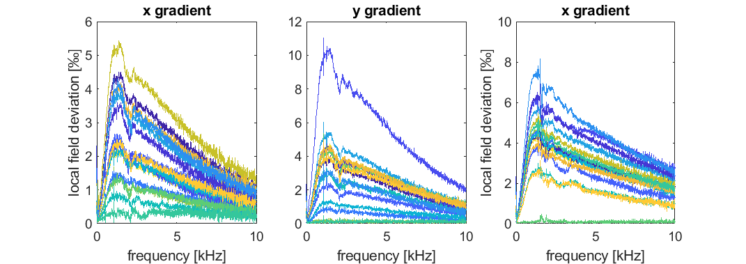
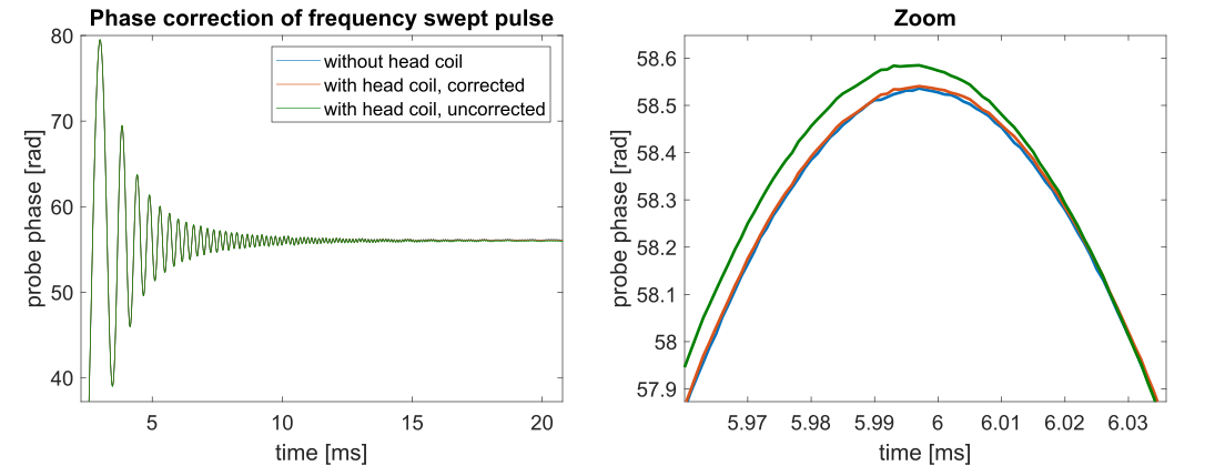
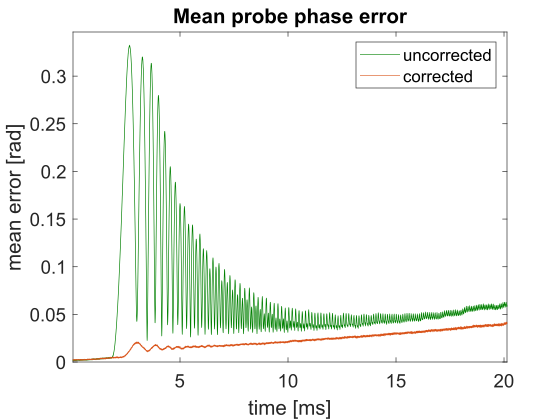
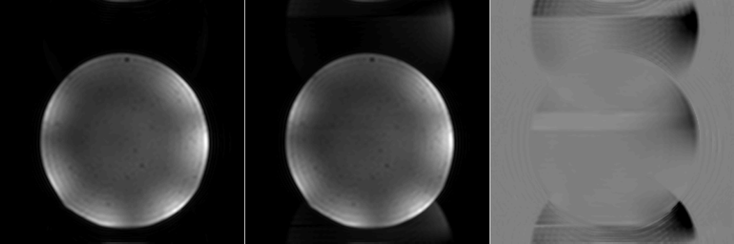
In Figure 1 the differences of the spectra of the gradient fields at the probe positions measured in presence and in absence of the head coil are shown. The effect amounts to several per mill of the maximal probe amplitude and concerns all probes. Figure 2 shows an example of a correction: the probe phase under a different frequency swept x-gradient was corrected. The result is summarized in Figure 3, which shows the mean remaining error of all corrections (with the mean taken over all three gradients and all probes), which is a lot smaller than the mean error without correction. Finally, Figure 4 shows that the ghost in an EPI reconstructed with a concurrently monitored trajectory vanishes when applying the correction.

Discussion and Conclusion

Erroneous probe signal due to local eddy currents induced by a head coil close to the probes can be effectively removed by convolving the signal with a transfer matrix. This one-time measurement correction enables now concurrent field monitoring of gradient sequences that were avoided because of this issue.

Acknowledgements

The authors thank Thomas Schmid for his support in the setup construction.