Introduction

The sound in MR-exams originates from the gradient coils and can be reduced by either switching the gradients very slowly or faster than the hearing threshold. Previously, we have presented a silent gradient axis that reduces the perceived sound during an exam by switching the gradient field at 20 kHz [1]. The silent gradient axis consists of a lightweight gradient insert that is positioned on the patient table, which produces a gradient field in the z-direction and is driven in synergy with the whole-body gradients. In this synergistic operation, the alignment of the silent gradient axis and whole-body z-gradient is important, as a misalignment produces phase-errors and results in image artifacts. In practice, this alignment of the two gradient axes is controlled by the patient table positioning system. We often observe that precise alignment is not always achieved. In this abstract, we show that the gradient point-spread function (PSF) can be used to retrospectively correct artifacts originating from the misalignment between the gradient insert and whole-body gradients.

Methods

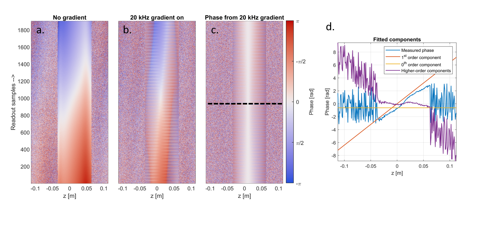
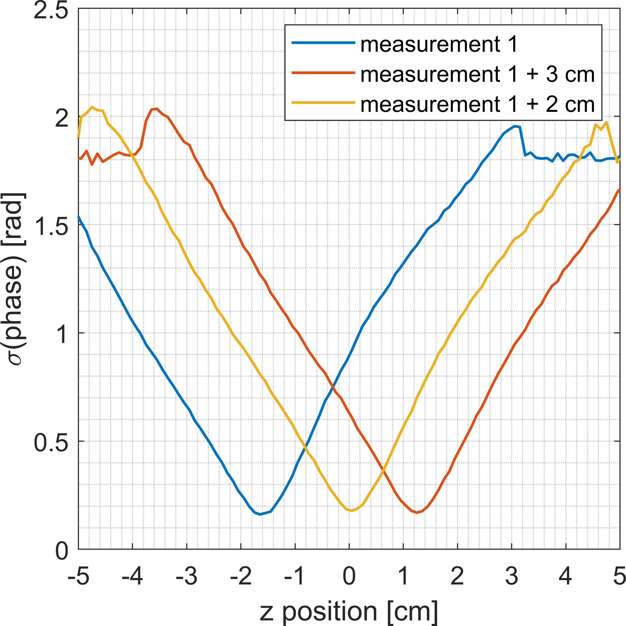
Gradient point-spread functions (further referred to as the PSF) are used in WAVE-CAIPI imaging to characterize the temporal behavior of fast-oscillating wave-gradients [2]. To acquire this PSF, two single-slice projections scans are needed, one with the oscillating gradient and one without [3]. During these scans, phase-encoding is only performed in the direction of the oscillating gradient (in our case the z-direction). After a 1D Fourier transform, the 1D spatial mapping of the accumulated phase over time is obtained (Figure 1a-c).

Three different PSF-mapping experiments, using different table positions, were performed to determine the accuracy of estimating the misalignment. Here, the displacement from a reference position was both measured with a ruler and using the PSF-mapping scans. In the PSF-mapping scans, the isocenter of the gradient insert was estimated by finding the position with the minimum standard deviation of the accumulated phase over time. The following imaging parameters were used in the PSF-mapping experiments: FOV= 224 mm, Voxel-size= 1 mm (both in the z-direction), slice thickness= 4 mm, the TE= 10.5 ms, TR= 30 ms and the flip angle= 26°.

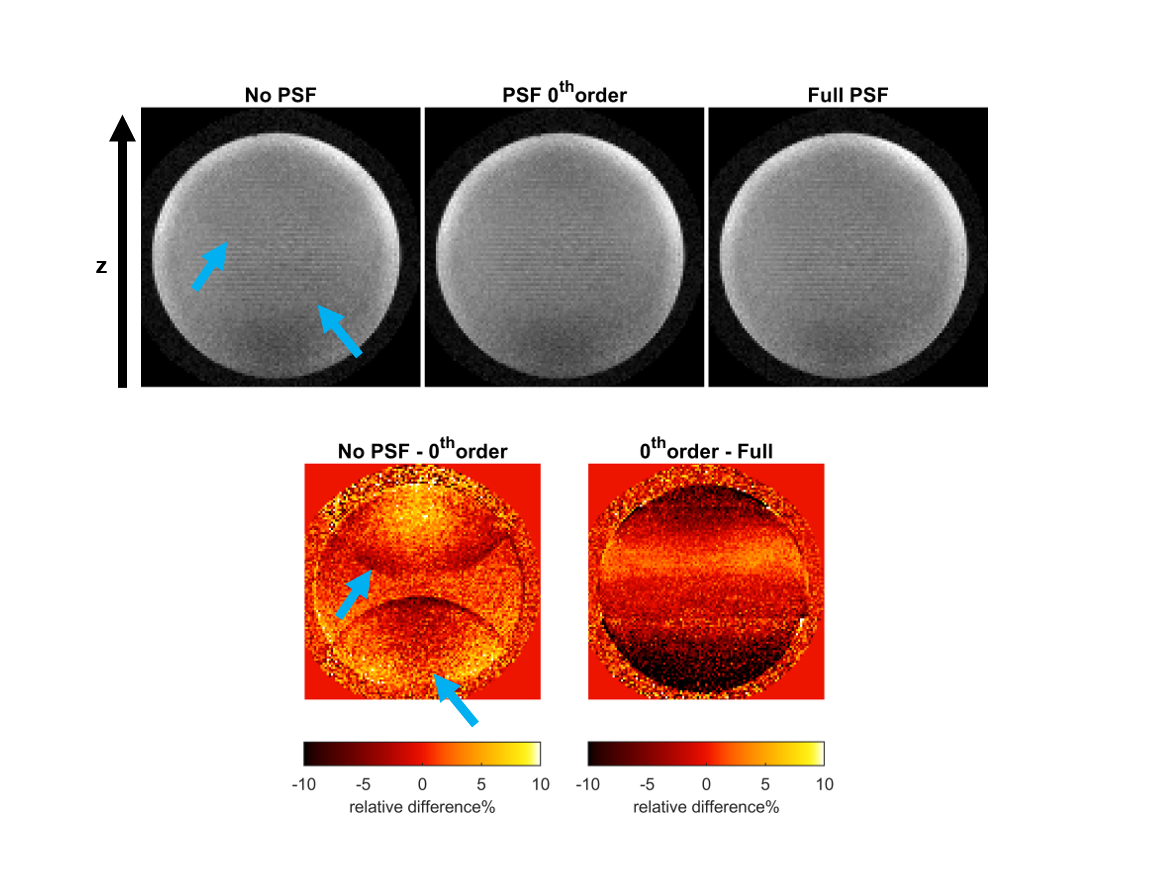
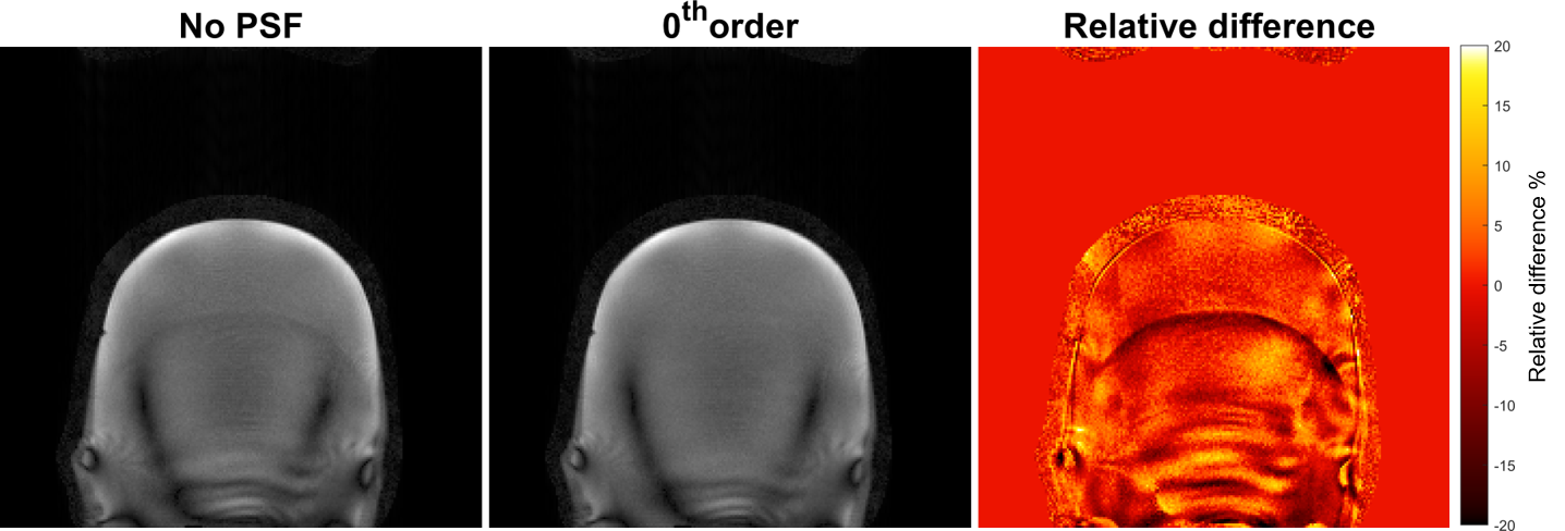
To test the misalignment correction, a spherical phantom (10-cm diameter) was imaged with a misalignment of 1 cm between the isocenter of the gradient insert and the whole-body z-gradient. Here, a modified 2D gradient-echo sequence was used in which the silent gradient axis was applied as an extra readout gradient in the phase-encoding direction. Here, only 53 phase-encoding lines were recorded, which was possible due to the extra spatial encoding provided by the silent gradient axis. The following imaging parameters were used: FOV= 224x224 mm², Voxel-size= 1x1 mm², slice thickness=4 mm, the TE= 10.5 ms, TR= 30 ms and the flip angle= 26°. This acquisition was repeated on a large head-shaped phantom with a misalignment of 2 cm.

Reconstruction and processing of the data was performed using an iterative SENSE reconstruction in MATLAB [4,5]. Three different misalignment corrections were compared for the reconstruction: without the PSF, with only the 0^th order spatial component of the PSF and with the full PSF (examples in Figure 1d). Here, the 0^th order spatial component was used to correct the phase of the signal in k-space. When using the full PSF, the 1^st order spatial component determined the k-space trajectory and the higher order components corrected the phase in a kx-z hybrid space (equivalent to what is used in WAVE-CAIPI reconstructions [2]).

For all experiments, the silent gradient axis was placed on the patient table of a 7T MR system (Philips, The Netherlands), operated at 28.6 mT/m (@20.2 kHz) and was fitted with a 32-channel receive coil (Nova Medical). An integrated birdcage coil was used for transmit.

Results and Discussion

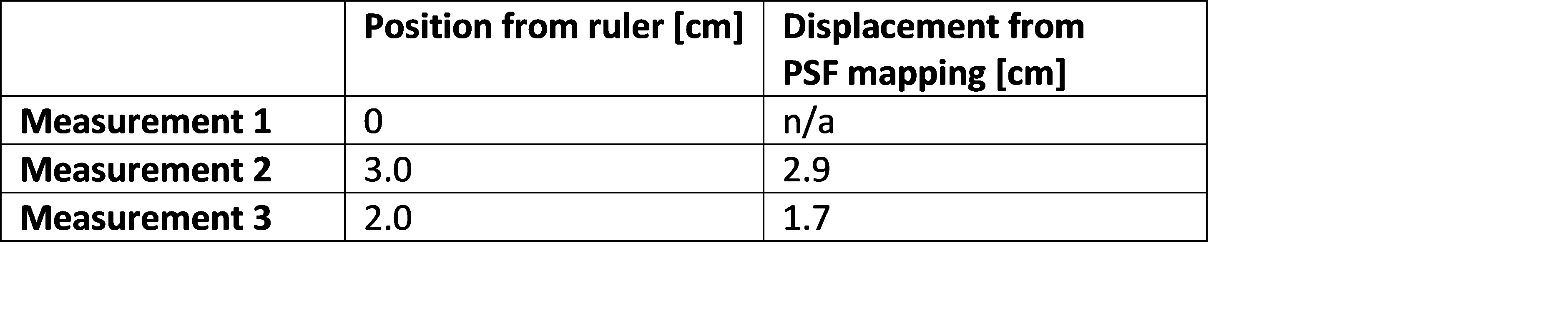
Figure 2 shows the curves used to estimate the table position and table 1 gives the table displacements that were estimated. Here, we can see that displacements measured using the ruler and using the PSF mapping match closely. Figure 2 also shows that the PSF-mapping scans could also be used as a tool to adjust the table-position online, as the measurement returns an estimation of the misalignment from with whole-body z-gradient. The precision of the estimated misalignment is determined by the resolution of the PSF-mapping scan (here 1 mm).

In the reconstruction without PSF (Figure 3), we see a ghosting artifact at the top and bottom of the phantom that disappears when applying the 0^th order component of the PSF. Applying the full PSF results in a more homogenous image but does not yield further reduction in the ghosting level. Therefore, the 0^th order component seems the most important for correcting misalignment artifacts as these 0^th order phase oscillations cause ghosting (displacement) artifacts. A scaled version of the same 0^th order component was applied, to accentuate the effect, to a large head phantom that also showed a reduction in ghosting artifacts (Figure 4).

Conclusion

We have shown that a gradient PSF-mapping experiment can be used to accurately determine the misalignment between a gradient insert and a whole-body gradient. This information can be used to correct images retrospectively, or do online adjustments to the table position and remove operator dependent image artifacts.

Acknowledgements

No acknowledgement found.