3087
Phantom-based high-resolution measurement of the gradient system transfer function1Department of Diagnostic and Interventional Radiology, University of Würzburg, Würzburg, Germany, 2Siemens Healthcare, Erlangen, Germany
Synopsis
The gradient system transfer function (GSTF) constitutes a comprehensive tool for correcting k-space trajectory distortions due to gradient infidelities. We developed a new phantom-based measurement approach that allows determining the GSTF with a high frequency resolution without relying on long readout durations. Our first results include self- and B0 cross-terms with high SNR and resolutions below 10 Hz, resolving the true width of several resonances. The high resolution enables us to capture long-lasting eddy current effects, which is especially promising for the application of GSTF-based correction methods in, for example, diffusion-weighted imaging.
Introduction
The gradient system transfer function (GSTF) can characterize the transmission behavior of the dynamic gradient system of an MR scanner and can be used to correct distorted k-space trajectories1. Two basic approaches for determining the GSTF have been reported before, namely the measurement with a field camera1 and a phantom-based method, which does not require additional hardware2. While the field camera can record the field evolution over extended time periods due to repeated excitation, the phantom-based method is limited by the T2*-decay of the MR-signal3. Consequently, the achievable frequency resolution of the phantom-based GSTF is limited as well. In this work, we present high-resolution GSTFs acquired with a new phantom-based measurement approach.Methods
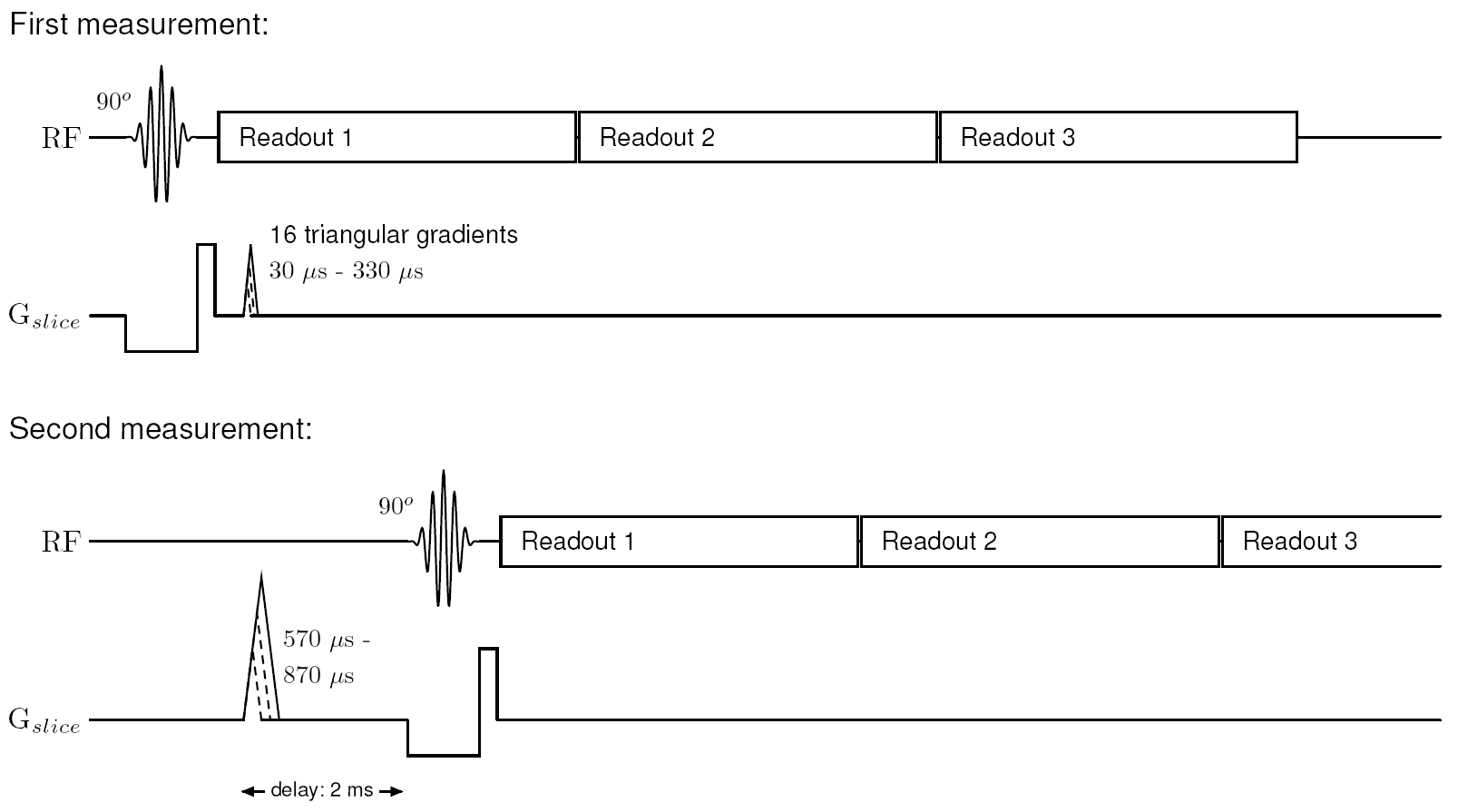
The measurements were conducted on a 3T Siemens MAGNETOM Prismafit scanner (Siemens Healthcare, Erlangen, Germany) using a 16-channel head coil and a spherical phantom. Sixteen triangular gradients of different durations were applied to achieve a high sensitivity at low frequencies and a broad spectral coverage of the input1. The gradient time course was measured with the thin-slice approach introduced by Duyn et al.4, using two slices of 3 mm thickness positioned at ±16.5 mm from the isocenter. Six different measurements were performed as follows. In the first measurement, the triangular gradient pulses were played out during the acquisition of the FID signal following a slice-selective excitation. In the remaining five measurements, the gradients were played out before the slice-selective excitation with delays of 2 ms, 22 ms, 42 ms, 62 ms and 82 ms between the start of the triangles and the excitation, respectively. In all measurements, the flip angle was 90° and TR was 1.0 s. Figure 1 schematically depicts the sequence timing of the first and second measurement. Exciting the phantom after application of the gradients enabled us to measure residual eddy current effects that persisted beyond the T2*-decay of the first measurement. The first measurement employed triangle durations between 30 µs and 330 µs and a slope of 180 T/m/s, while the other measurements used triangle durations between 570 µs and 870 µs and slopes of 150 T/m/s (z-axis and x-axis) or 130 T/m/s (y-axis). These longer triangles covered a narrower bandwidth but provided a higher sensitivity between –3 kHz and 3 kHz. In the first measurement, they would have completely dephased the signal. Each measurement comprised three consecutive signal readouts of approximately 25 ms, yielding a total readout duration of approximately 75 ms after each excitation. The combination of all six measurements thus covered a total time window of approximately 157 ms. The GSTF was calculated by solving a linear system similar to the method recently proposed by Wilm et al.5 and Fourier transforming the result.Results
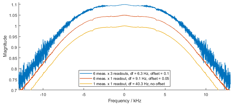
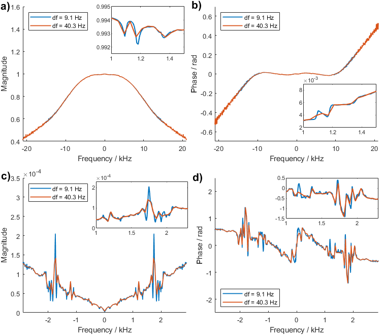
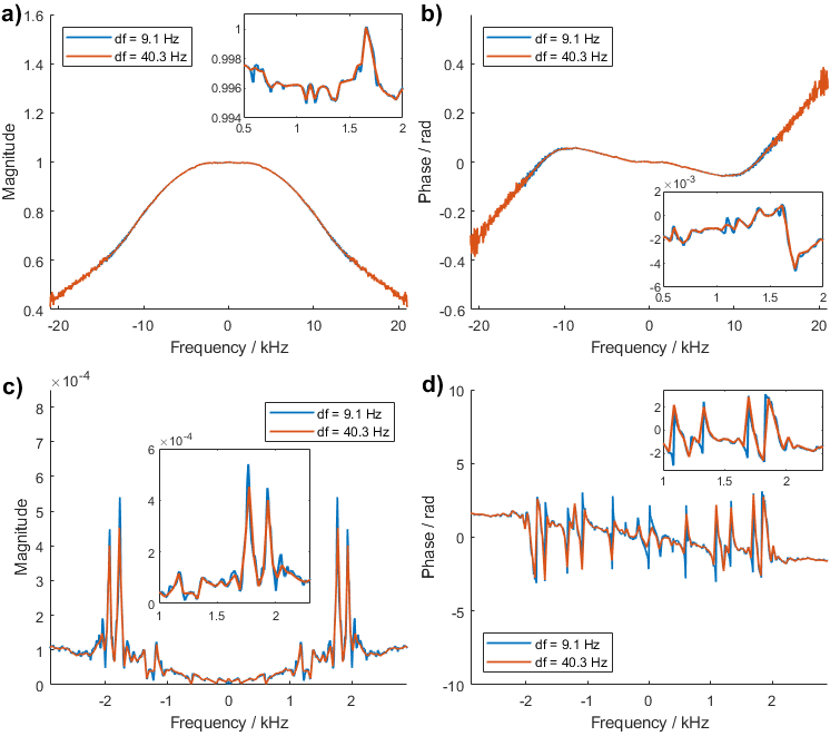
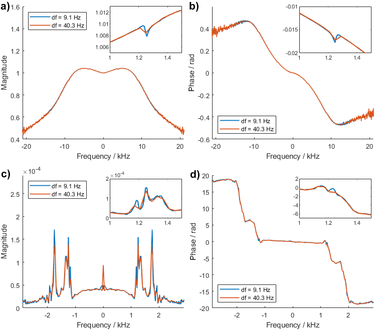
Figure 2 displays the self-term of the GSTF in x-direction calculated from three differently sized datasets. The curve with the highest frequency resolution of 6.3 Hz, determined from the full-sized dataset, exhibits an undesirably high noise level, caused by the low SNR in the second and third readout of each measurement. The noise can be alleviated by using only the first readout of each measurement for the calculation, which still yields a resolution of 9.1 Hz. When evaluating only the first readout of the first measurement, the SNR is comparable but the achieved frequency resolution is only 40.3 Hz. Figures 3, 4 and 5 display the magnitude and phase of the self- and 0th-order cross-term of the GSTFs in x-, y- and z-direction with two different frequency resolutions, namely 9.1 Hz and 40.3 Hz. The insets in the figures show closer views of different resonance peaks. It is clearly visible that the lower frequency resolution of 40.3 Hz cannot resolve the true widths of all resonances, for example in Figure 3a), c) or Figure 5a), b), c). Some resonances do not appear at all when the frequency resolution is only 40.3 Hz, as for example in Figure 3d) around 1.2 kHz, in Figure 4a) around 0.6 kHz or in Figure 5d) around 1.25 kHz.Discussion
The width of a resonance in the GSTF is inversely proportional to the lifetime of the respective eddy current effect. Measuring the GSTF with a high frequency resolution is thus especially vital for corrections of long-lasting eddy current effects, as occurring for example in diffusion-weighted imaging6. Our new measurement approach allows this even when the signal decays quickly and thus prohibits long readout durations, as demonstrated by our GSTF measurements in x-direction. We chose the linear system approach for calculating the GSTF because it is a convenient method for combining several measurements with different input gradients. Furthermore, we used triangular test gradients instead of a chirp-waveform7 to avoid ringing artifacts in the GSTF. Knowledge of the GSTF allows for a comprehensive correction of various k-space trajectories, especially non-Cartesian ones2,7, either in post-correction2 or by a gradient pre-emphasis8.Conclusion
In this work, we present a new phantom-based measurement approach for the GSTF that is independent from the T2*-signal decay and show first GSTFs with a high frequency resolution of 9.1 Hz that were acquired using only a large phantom and the scanner hardware.Acknowledgements
No acknowledgement found.References
1. Vannesjo SJ, Haeberlin M, Kasper L, et al. Gradient System Characterization by Impulse Response Measurements with a Dynamic Field Camera. Magn Reson Med. 2013;69:583-593.
2. Addy NO, Wu HH, Nishimura DG. Simple Method for MR Gradient System Characterization and k-Space Trajectory Estimation. Magn Reson Med. 2012;68:120-129.
3. Graedel NN, Hurley SA, Clare S, et al. Comparison of gradient impulse response functions measured with a dynamic field camera and a phantom-based technique. In ESMRMB 2017, 34th Annual Scientific Meeting, Barcelona, ES, October 19–October 21: Abstracts, Saturday. Magn Reson Mater Phy. 2017;30:361-362.
4. Duyn JH, Yang Y, Frank JA et al. Simple Correction Method for k-Space Trajectory Deviations in MRI. J Magn Reson. 1998;132:150-153.
5. Wilm BJ, Dietrich BE, Reber J, et al. Gradient Response Harvesting for Continuous System Characterization During MR Sequences. IEEE Trans Med Imag. 2020;39(3):806-815.
6. Papadakis NG, Martin KM, Pickard JD, et al. Gradient Preemphasis Calibration in Diffusion-Weighted Echo-Planar Imaging. Magn Reson Med. 2000;44:616-624.
7. Kronthaler S, Rahmer J, Börnert P, et al. Trajectory correction based on the gradient impulse response function improves high-resolution UTE imaging of the musculoskeletal system. Magn Reson Med. 2020;00:1-15.
8. Stich M, Wech T, Slawig A, et al. Gradient waveform pre-emphasis based on the gradient system transfer function. Magn Reson Med. 2018;80:1521-1532.
Figures