Introduction

Field perturbations caused by eddy currents induced in gradient coils and conducting structures, mechanical oscillations and fluctuations due to fast gradient switching are well known sources of image artifacts, compromise gradient performance, and impact MR image interpretations. In previous studies, field monitoring with a dynamic field camera, has demonstrated improved image quality¹. However, field monitoring is limited by fast decay times of the probes (T₂=35ms, signal lifetime~50ms), with simultaneous measurements requiring the probes to either be integrated with the primary phased-array receiver coil, complicating patient set-up or to be performed in a separate scan session causing system interruptions.
A practical alternative is to characterize gradient performance by using an impulse response function (IRF), allowing deviations of the target gradient waveforms to be corrected. Utilizing linear systems theory, the gradient system can be approximated as linear time-invariant (LTI), providing a method to estimate system performance and to predict arbitrary waveforms and trajectories. This approach has previously been proposed in several studies^2-3, where short field measurements with known inputs were used. In this study a field monitoring system¹ (Skope, Zurich, Switzerland) was used to characterize the gradient IRF, for a high-performance head-only gradient⁴. The use of a field monitoring system, with multiple probes allows the decomposition of the spatial response into higher order spherical harmonics, providing higher order and cross-term information. Preliminary experimental results highlighting calibration and performance of the gradient IRF are presented.

Methods

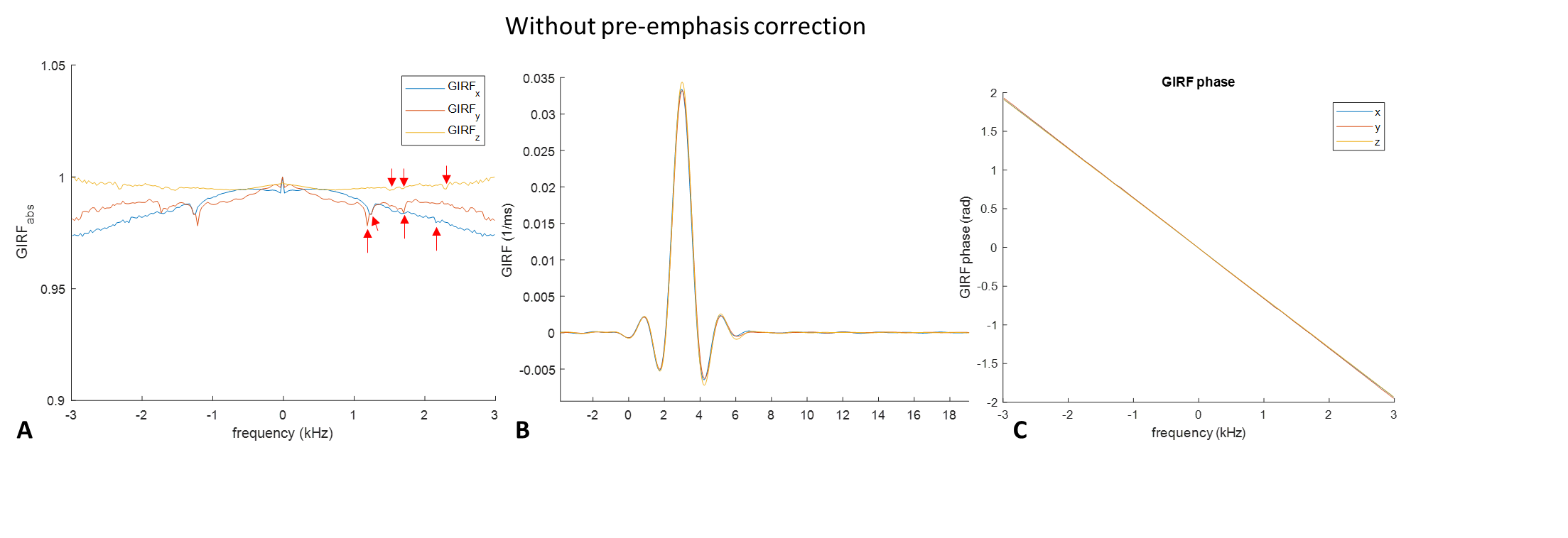
Field measurements were performed on a whole-body 3T magnet (GE SIGNA MR750), equipped with a high-performance head-only gradient (MAGNUS)⁴ achieving 200mT/m and 500T/m/s with a standard 1MVA gradient driver. Triangular waveforms (Figure 1), providing a close surrogate to delta functions were used to probe the system response. A combination of ~60 waveforms, individually applied to each axis, with rise times ranging between 31-320ms were used, while maintaining the field cameras dynamic range. Field outputs were collated² to yield the IRF using, $$ IRF(ω)= (∑Input_j^* (ω) Output_j (ω))/(∑|Input_j (ω)|^2 )$$

Data was acquired without pre-emphasis compensation. As the MAGNUS gradient has asymmetric transverse gradient axes (x-y), associated zeroth and first order concomitant gradient are present. The IRF measurement included these, as well as second order concomitant fields (also present in fully symmetric gradient coils).
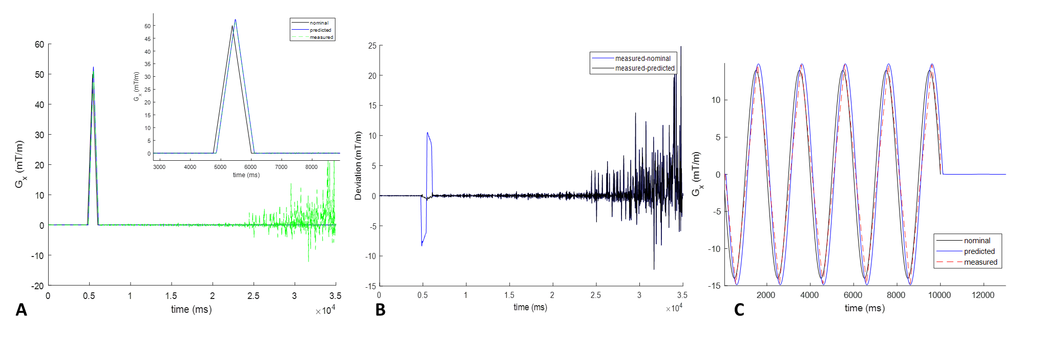
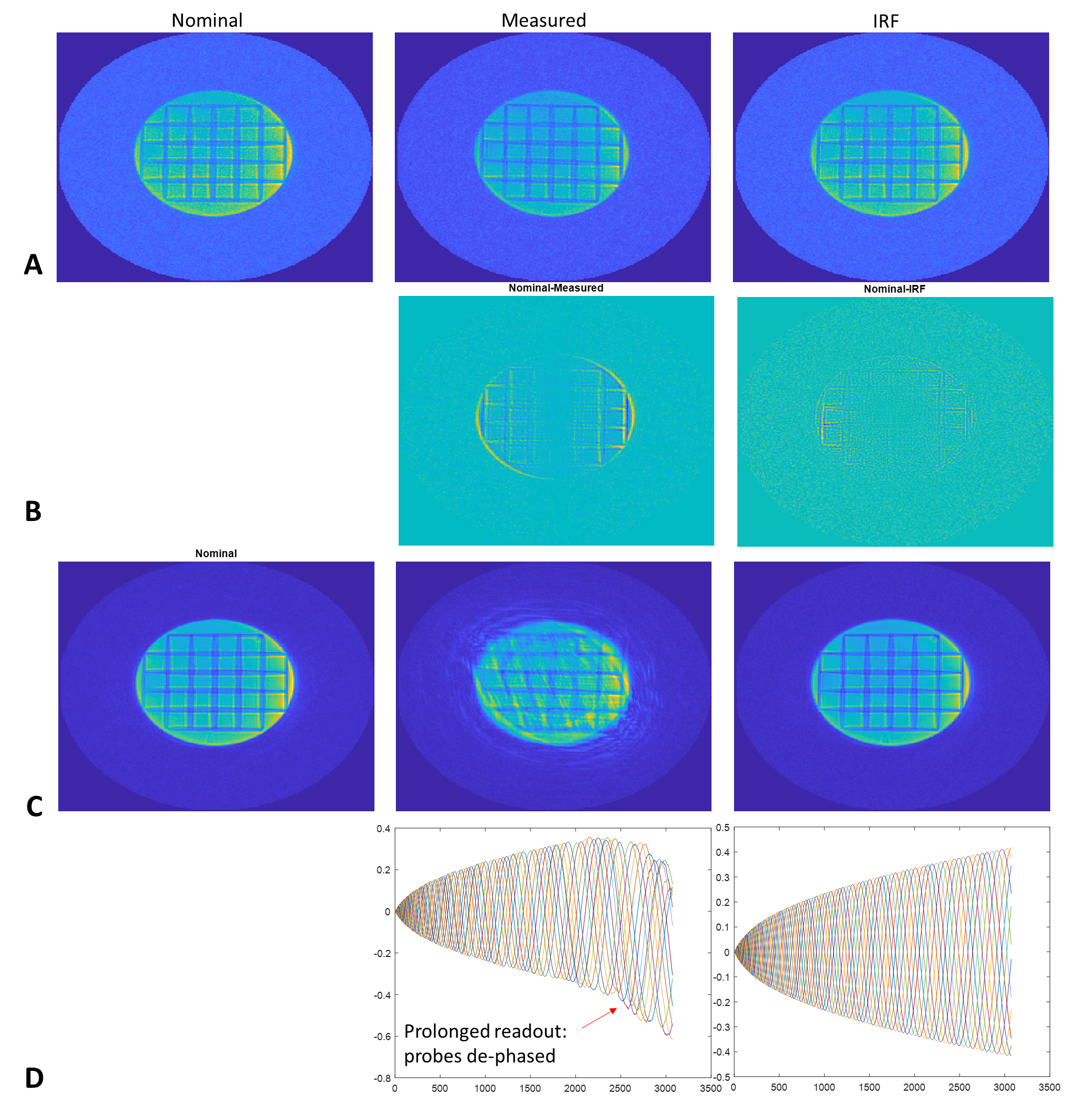
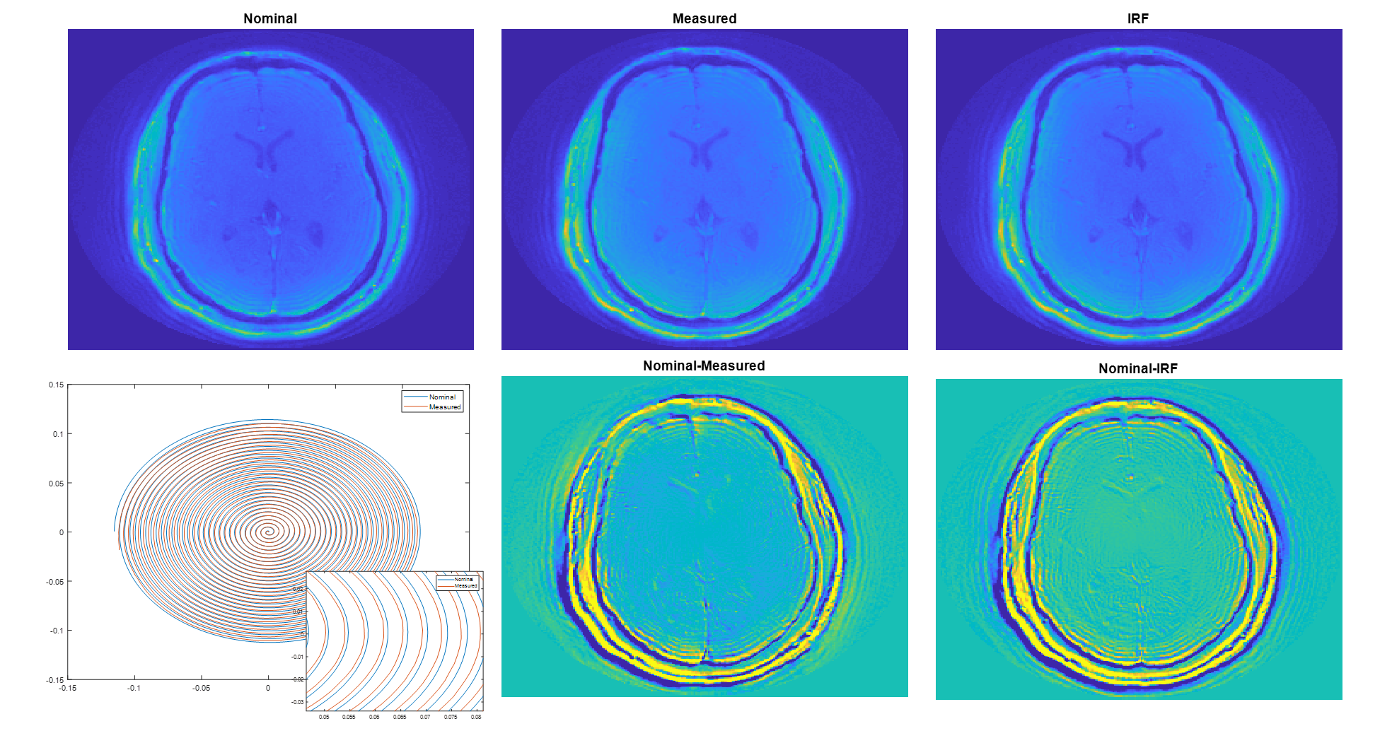
For validation, IRF predictions were used to estimate arbitrary waveforms by comparing predictions to nominal and field-monitored measurements. For this, sinc and triangle waveforms were chosen. To estimate trajectories, a 2D single-slice spiral with SR =156T/m/s, 3072 points, and TE/TR=2.4/25ms was acquired on a small grid-phantom and in a healthy volunteer (under an IRB approved protocol) with a total readout time of 3ms per spiral interleave arm. k-space trajectory prediction from the IRF, obtained by time domain convolution with the nominal gradient input, was used for regridding non-cartesian k-space data. The reconstructed images were compared to reconstruction with nominal trajectories as well as using the measured trajectories (using field monitoring).

Results and Discussion

Channel specific mechanical oscillations in the IRF with distinct peaks at <1% of the full response, were noted (Figure 2). The time domain representation highlights the system delay without pre-emphasis correction. In addition to delay times, the IRF is also able to capture subtle mechanically induced field oscillations. Error plots (Figure 3) highlight correspondence between the IRF prediction and field monitored approach for two arbitrary input waveforms. The correspondence between IRF predicted and monitored trajectory correction is highlighted with phantom (Figure 4 A/B) in vivo trajectory-based reconstructions (Figure 5).
Interestingly, strong aliasing is not visible even with the nominal reconstruction, for both phantom and in vivo implementations potentially attributable the systems eddy current profile (design specs <0.05%). The benefit of the IRF prediction is realized for acquisitions with longer readouts, where monitoring is limited by probe dephasing (Figure 4 C&D), but adequate compensation can be achieved with the predicted trajectories.
Residual artifacts are potentially due to the absence of active compensation for linear (and higher order) components of the concomitant field as well as static off resonance, which can be compensated with B₀ correction. Furthermore, the clip-on sensors cover the edge of the imaging volume, where for a small head gradient with a design 26 cm FOV for linearity and uniformity, measurements are dependent on the accurate positional determination of the sensors. Errors in position calibration, or even displacement of the clip-ons can contribute to errors.

Conclusions

Unlike concurrent field monitoring, the IRF needs to be determined once for a system, providing a practical method to not only tune pre-emphasis, but account for mechanically induced oscillations and correct for gradient imperfections. From an image reconstruction perspective, the predicted trajectories can be actively incorporated for real time correction, without scanner downtime. Furthermore, the predicted waveforms and trajectories demonstrate equivalent correction to the field monitoring system. Though an improvement to image quality is apparent, this approach needs to be further tested for a wider range of implementations, such as incorporating higher order field terms to refine or thermal effects to test departure from the LTI approximation.

Acknowledgements

Grant funding from NIH U01EB28976, CDMRP W81XWH-16-2-0054