3084
High resolution in-vivo relaxation time mapping at 50 mT.1C.J. Gorter Center for High Field MRI, Leiden University Medical Center, Leiden, Netherlands
Synopsis
Recent years have seen a renewal in interest in low field MRI systems due to its lower cost, increased portability and robustness to medical implants, with the obvious disadvantage of lower SNR compared to clinical high field systems. In this work we present T1 and T2 relaxation maps of the brain and lower leg to facilitate the optimization of sequence parameters. Generally the T1 times are shorter and T2 times are slightly longer than at clinical field strengths.
Introduction
Several recent publications have shown the promise of very low field MRI of the brain and extremities using Halbach (1), double-planar (2, 3), modified Halbach (4) and field-cycling magnets (5). Low field MRI has many advantages over its higher field counterpart including ease of siting, purchase and maintenance costs, and robustness with respect to medical implant contraindications (6). The major disadvantage is of course a lower contrast-to-noise ratio (CNR). However, some of this CNR-loss can be regained by the judicious use of appropriate pulse sequences (7) taking advantage of favourable relaxation times at lower field, as well as more efficient data collection with TSE sequences due to the much lower specific absorption rate (SAR). In order to optimize sequence parameters, relaxation times need to be characterized and in this work we measure in-vivo relaxation times of several tissue types across different subjects using a 50 mT low-field scannerMethods
The Halbach array has been described in detail in previous publications (1). The MRI scanner operates at 50.4 mT and has a clear bore of 27 cm, and a length of 50 cm. For head imaging a 24x18x15 cm elliptical solenoid coil with 25 turns was used as a transmit/receive coil, for leg imaging a 15 cm diameter, 15 cm long solenoid with 57 turns was used. A Magritek Kea2 spectrometer (Aachen, Germany) was used to generate gradient wave forms and RF pulses as well as digitising the generated echoes. The RF pulses generated were amplified by a custom built 1 kW RF amplifier and a custom built 3 axis gradient amplifier was used to drive the gradient coils. For in vivo imaging the section of the torso extending out of the Faraday shield was wrapped in a conductive fabric grounded to the Faraday cage to reduce external electromagnetic interference. In vivo imaging experiments.All data were acquired with a bandwidth of 20 kHz, with 90 and 180o RF pulse length of 100 us. Raw k-space data was filtered using a sine-bell-square filtered before reconstructing using an FFT. Relaxation data were fitted to a single exponential recovery curve on a pixel-by-pixel basis in python using the least squares fitting algorithm in the Scipy package.
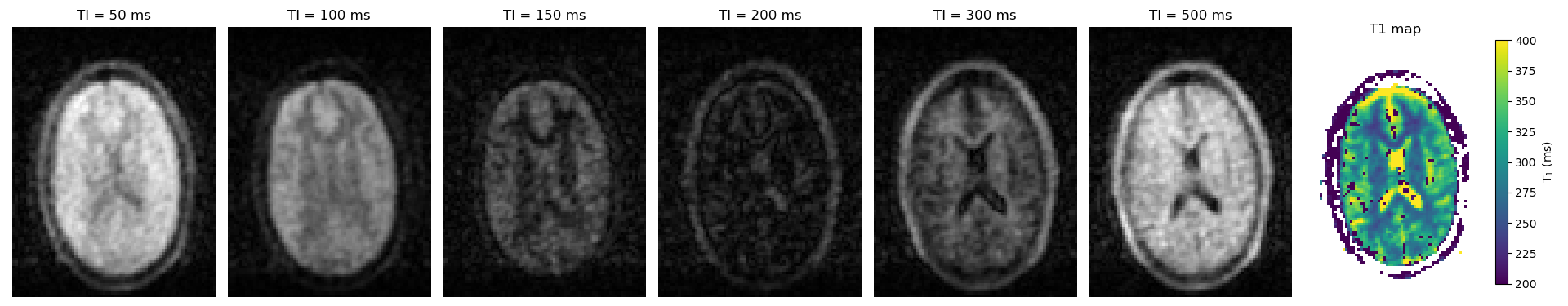
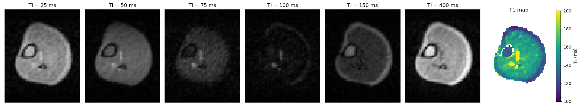
T1 mapping was performed using a 3D Inversion recovery sequence with TSE readout with a low-high k-space trajectory. Brain data were acquired with the following parameters: FoV: 240x180x150mm, resolution: 2.5x2.5x5mm, inversion times: 50, 100, 150, 300, 500 ms, TR/TE: 1250/13 ms, echo train length: 6. Data on the lower leg were acquired with the following parameters FoV: 150x130x150 mm, resolution: 2.5x2.5x5mm, inversion times: 25, 50, 75, 100, 150, 400 ms, TR/TE: 1200/11 ms, echo train length: 3.
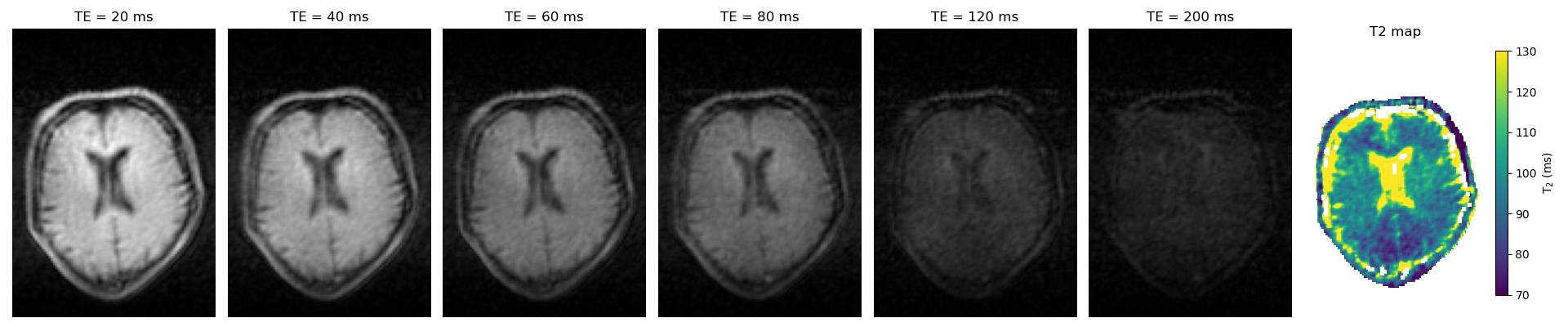
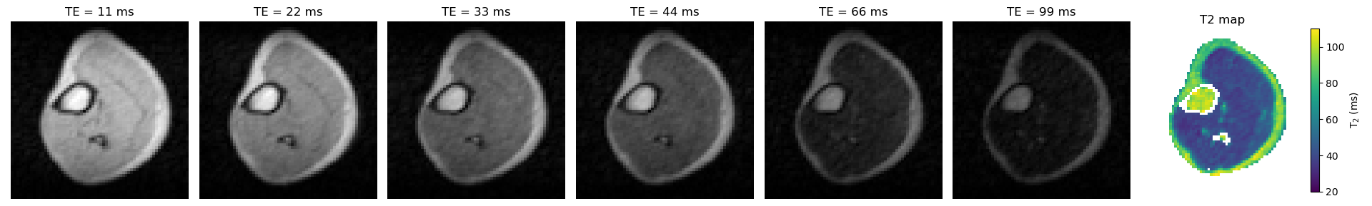
T2 mapping was performed using a 3D multi-echo spin-echo sequence with 10 echoes. Data on the brain were acquired with the following parameters: FoV: 250x180x180 mm, resolution: 2x2x5 mm, echo spacing: 20 ms, TR: 750 ms. Data on the lower leg were acquired with the following parameters: FoV: 128x128x120 mm, resolution: 2x2x6 mm, echo spacing: 11 ms, TR: 800 ms. Data was correcting for temperature-induced B0 during the acquisition by phase shifting k space in post processing. All data were acquired on healthy volunteers.
Results
Figure 1 shows a transverse slice of the brain from the 3D dataset at six different inversion times and the generated T1 map. Values are averaged over different tissue-type voxels, and reported with a calculated standard deviation. Figure 2 shows corresponding brain data for six different echo times and a T2 map reconstructed from the images. In both cases the CSF appears hypointense due to saturation from the long T1 (>1500 ms) and relaxation times are therefore not calculated. Figure 3 shows images of a transverse slice in the calf muscle acquired with different inversion times and a T1 map generated from the data. Figure 4 shows a single slice reconstructed at different echo times from a multi-echo spin echo sequence acquired on the lower leg and a T2 map generated from the data.Discussion
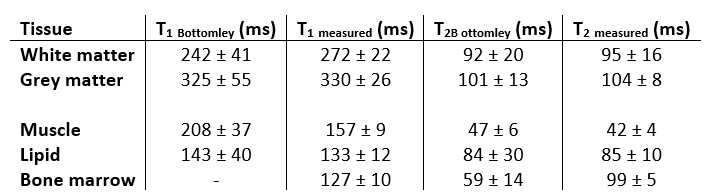
In this work we show that image quality and SNR on a custom-built 50 mT MRI scanner are sufficient to produce high quality relaxation maps in different tissues. Figure 5 shows a table of the measured relaxation times compared to classic (ex-vivo) literature values. Relaxation times for the brain agree very well, with slightly higher values for muscle T1 and bone marrow T2 (note that at higher fields bone marrow T2 values are consistently reported as being higher than lipid, in line with our measured values). As expected the measured T1 relaxation times are shorter than those at clinical field strength of 1.5 and 3 Tesla (9) while the T2 values are generally slightly longer, probably due to local microsusceptibility effects . The small difference in T1 and T2 between grey and white matter also suggest that generating good contrast between the two tissues will be challenging at low field, and other approaches may have to be investigated such as magnetisation transfer or diffusion weighted imaging.Acknowledgements
This work is supported by the following grants: Horizon 2020 ERC FET-OPEN 737180 Histo MRI, Horizon 2020 ERC Advanced NOMA-MRI 670629, Simon Stevin Meester Award and NWO WOTRO Joint SDG Research Programme W 07.303.101.References
1. O'Reilly T, Teeuwisse WM, de Gans D, Koolstra K, Webb AG. In vivo 3D brain and extremity MRI at 50 mT using a permanent magnet Halbach array. Magn Reson Med. 2020.
2. He Y, He W, Tan L, Chen F, F. M, Feng H, et al. Use of 2.1 MHz MRI scanner for brain imaging and its preliminary results in stroke. J Magn Reson. 2020;319:106829.
3. Sheth KN, Mazurek MH, Yuen MM, Cahn BA, Shah JT, Ward A, et al. Assessment of Brain Injury Using Portable, Low-Field Magnetic Resonance Imaging at the Bedside of Critically Ill Patients. Jama Neurol. 2020.
4. Cooley CZ, McDaniel P, Stockmann J, Srinivas SA, Cauley SF, Sliwiak M, et al. A portable brain MRI scanner for underserved settings and point-of-care imaging. arXiv:200413183 [eessIV]. 2020.
5. Broche LM, Ross PJ, Davies GR, Macleod MJ, Lurie DJ. A whole-body Fast Field-Cycling scanner for clinical molecular imaging studies. Sci Rep-Uk. 2019;9.
6. Sarracanie M, Salameh N. Low-Field MRI: How Low Can We Go? A Fresh View on an Old Debate. Front Phys-Lausanne. 2020;8.
7. Marques JP, Simonis FFJ, Webb AG. Low-field MRI: An MR physics perspective. J Magn Reson Imaging. 2019;49(6):1528-42.
8. Bottomley PA, Foster TH, Argersinger RE, Pfeifer LM. A Review of Normal Tissue Hydrogen Nmr Relaxation-Times and Relaxation Mechanisms from 1-100 Mhz - Dependence on Tissue-Type, Nmr Frequency, Temperature, Species, Excision, and Age. Med Phys. 1984;11(4):425-48.
9. Korb JP, Bryant RG. Magnetic field dependence of proton spin-lattice relaxation times. Magn Reson Med. 2002;48(1):21-6.
Figures