3083
T1 quantification in fast field-cycling MRI using model-based reconstruction1Graz University of Technology, Graz, Austria, 2Institute of eHealth, University of Applied Sciences FH JOANNEUM, Graz, Austria, 3BioTechMed Graz, Graz, Austria, 4Acute Stroke Unit, Aberdeen Royal Infirmary, Aberdeen, United Kingdom, 5Aberdeen Biomedical Imaging Centre, Univeresity of Aberdeen, Aberdeen, United Kingdom
Synopsis
T1 maps from fast field-cycling (FFC) MRI can provide insights to structural information and dynamics of molecular system not accessible by traditional MRI. The low SNR associated with the lower field strength in FFC imaging (0.2 T - 50 µT) leads to long acquisition times, impairing its clinical applicability. Hence, we propose a model-based reconstruction strategy to reduce acquisition time and improve image quality of multi-field T1 maps. The method is compared to standard fitting on numerical phantoms and a in vivo stroke patient. Model-based reconstruction clearly outperformed standard fitting, reducing noise and revealing previously unseen details in low-field T1 maps.
Indroduction
Fast field-cycling (FFC) is a technique that consists in changing rapidly the main magnetic field of MRI systems1 and is mostly used to investigate the field dependent changes of longitudinal relaxation times ($$$T_1$$$), also referred to as $$$T_1$$$ Nuclear Magnetic Relaxation Dispersion (NMRD)3,4. NMRD profiles can provide insights to underlying structural information and dynamics of molecular systems but can not be accessed by traditional MRI systems5,6,7,8.Recently, a whole-body FFC system has been developed and approved for clinical studies, allowing multi-field $$$T_1$$$ mapping at any field from 50 μT to 0.2 T2. This opens new prospects for clinical research but in vivo applications are limited by low SNR inherent to the lower field strength, potentially combined with a small dispersion signal9, leading to a long scan time. To this end, we propose a model-based reconstruction approach to quantify $$$T_1$$$ from multi-field FFC data, which had been previously shown to provide high quality quantitative maps in high-field applications10,11,12. The proposed method is tested on simulated head phantoms and subsequently applied to in vivo FFC data of a patient suffering from a stroke. Fitted $$$T_1$$$ maps are compared to results from a Tikhonov regularized, non-linear least squares (NLLS) approach13,14, applied to the complex imagedata.Theory
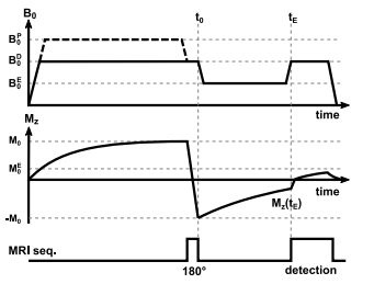
Quantifying $$$T_1$$$ with FFC methods can be achieved by means of an inversion recovery sequence, including field switching during the inversion time, called evolution time ($$$T_E$$$) in FFC imaging15 (see Figure 1). The signal intensity ($$$S_{B_0^E,t^E}$$$) for such a sequence is governed by$$S_{B_0^E,t_E}(u:=(C,T_{1}^{E})) = C\,[-\alpha_{B_0^E} \,B_0^D\,e^{\frac{-t_E}{T_{1}^{E}}} + B_0^E\,(1-e^{\frac{-t_E}{T_{1}^E}})]$$
with $$$C$$$ being proportional to proton density. $$$T_1^E$$$ describe the field dependent relaxation. $$$\alpha_{B_0^E}$$$ accounts for imperfections of inversion pulse and field ramping. The signal equation is combined with the Fourier and sampling operator $$$\mathcal{F}$$$ to directly quantify $$$T_1$$$ from complex k-space data. Joint spatial TGV16,17 constraints are posed on the unknown quantitative maps, utilizing common information between the maps18,19. This leads to the following optimization problem
$$\underset{u,v}{\min}\quad \frac{1}{2}\sum_{i=1}^{N_E}\sum_{n=1}^{{N_t^{E_i}}}\|\mathcal{F}S_{B^{E_i}_0,t^{E_i}_n}(u)-d_{n,i}\|_2^2 + \gamma( \alpha_0\|\nabla u - v\|_{1,2,F} + \alpha_1\|\mathcal{E}v\|_{1,2,F})$$
with $$$N_E$$$, $$$N_t^{E_i}$$$ and $$$d_{n,i}$$$ standing for the number of magnetic field strengths probed, the number of inversion times for each field and the NMR signal data acquired, respectively. $$$\mathcal{E}$$$ approximates the 2nd-order derivative and auxiliary variable $$$v$$$ balances between 1st and 2nd derivative. This problem is solved using a recently proposed model-based reconstruction framework20.
Methods
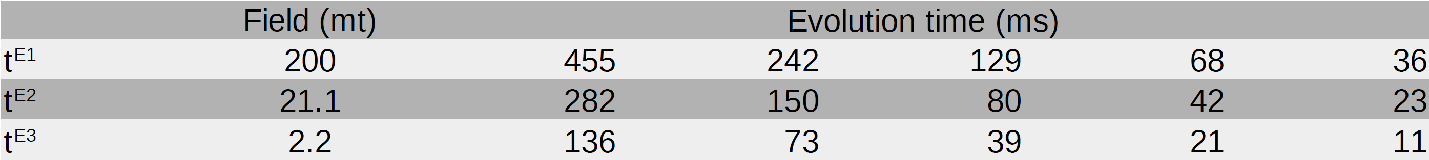
The simulated phantom consisted of five regions mimicking the dispersive characteristics of an axial head scan: subcutaneous fat (ROI-1), tissue surrounding the brain (ROI-2), the brain (ROI-3), and a stroke-like lesion (ROI-4). The image resolution was chosen as 90x90 voxels; simulated evolution times and fields are given in Table 1. To simulate noise, complex-valued Gaussian noise with a standard deviation of four percent of the highest signal as added to the images. The in vivo brain data was selected from the PUFFINS study (Potential Use of Fast Field-cycling IN Stroke), a pilot study for the imaging of acute brain stroke by FFC imaging currently taking place at the University of Aberdeen and approved by the local Ethics Committee (NoSREC reference 16/NS/0136/AM01). Informed consent was given by all participants. The acquisition was performed on a patient with right occipital infarct (previously validated by CT scan) using a whole-body FFC scanner with an adapted inversion-recovery spin echo sequence. The image size was 128x128 with 10 mm slice thickness, 62.5% partial Fourier, 29 kHz bandwidth, 290mm FOV and pre-polarisation at 200 mT for 300ms. Total acquisition time was 40 minutes. Evolution times were the same as in the numerical simulation.Results
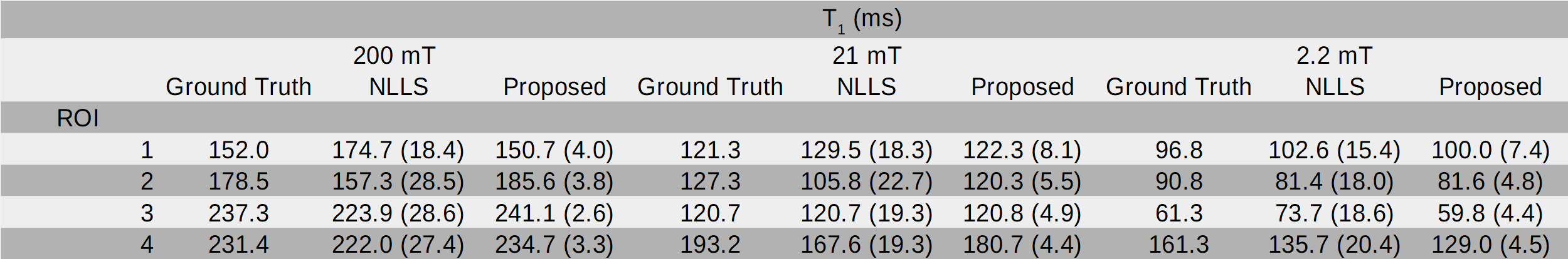
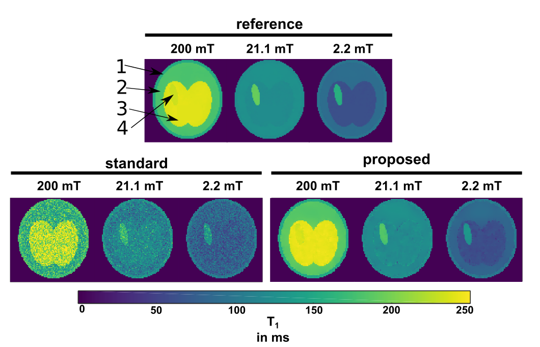
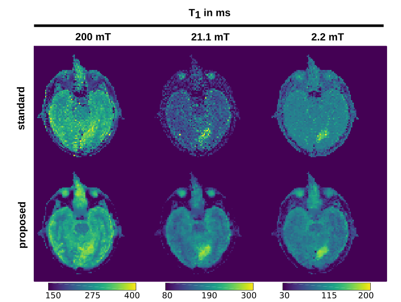
Applying the proposed method on the simulated data gave cleaner $$$T_1$$$ maps compared to standard fitting (NLLS, see Figure 1). Quantitative values for ROIs 1-4 are given in Table 2, showing a decrease in standard deviation for the proposed method. The in vivo results are given in Figure 2: again, the proposed method reduced the noise in the image compared with standard voxel-wise fitting, even showing some structural details of the brain in the 21.1 mT images. The stroke can be clearly delineated in the smaller fields. The algorithm ran an NVIDIA Geforce GTX 1080 TI and fitting took ~3 minutes for the shown $$$T_1$$$ maps.Discussion
The model-based reconstruction approach proposed, combined with the joint spatial TGV regularization, clearly outperforms the current standard of voxel-wise $$$T_1$$$ fitting dispersion maps of FFC data. Due to the redundant information present in the FFC imaging technique, a joint regularization approach fully utilizes the available information in the data. This reveals previously unseen structures, hidden in noise, in high as well as low field $$$T_1$$$ maps (Figure 3). Poor SNR can lead to a bias in both methods but the proposed method stays generally closer to the true values and offers a huge decrease in standard deviation. Selecting smaller regularization weights lead to smaller bias at the expense of increased noise in the reconstructed images. The framework used here can be readily extended to a multi-coil setting or to non-Cartesian sampling strategies to speed up the acquisition of FFC imaging in the future. This shows exciting potential for the exploration of low magnetic fields and $$$T_1$$$ dispersion effects as illustrated here on a stroke patient.Acknowledgements
Oliver Maier acknowledges grant support from the Austrian Academy of Sciences under award DOC-Fellowship 24966.
The authors would like to acknowledge the NVIDIA Corporation Hardware grant support.
References
[1] Bödenler M, de Rochefort L, Ross PJ, Chanet N, Guillot G, Davies GR, et al. Comparison of fast field-cycling magnetic resonance imaging methods and future perspectives. Molecular Physics 2019 apr;117(7-8):832–848. https://doi.org/ 10.1080/00268976.2018.1557349.
[2] Broche LM, Ross PJ, Davies GR, MacLeod MJ, Lurie DJ. A whole-body Fast Field-Cycling scanner for clinical molecular imaging studies. Scientific Reports 2019;9(1):10402. https://doi.org/10.1038/s41598-019-46648-0.
[3] Steele RM, Korb JP, Ferrante G, Bubici S. New applications and perspectives of fast field cycling NMR relaxometry. Magnetic Resonance in Chemistry 2016;54(6):502–509.
[4] Korb JP. Multiscale nuclear magnetic relaxation dispersion of complex liquids in bulk and confinement. Progress in Nuclear Magnetic Resonance Spectroscopy 2018 feb;104:12–55. https://www.sciencedirect.com/science/article/ pii/S0079656517300353.
[5] Broche LM, Ismail SR, Booth NA, Lurie DJ. Measurement of fibrin concentration by fast field-cycling NMR. Magnetic Resonance in Medicine 2011 oct;67(5):1453–1457. https://doi.org/10.1002/mrm.23117.
[6] Broche LM, Ashcroft GP, Lurie DJ. Detection of osteoarthritis in knee and hip joints by fast field-cycling NMR. Magnetic Resonance in Medicine 2012;68(2):358–362.
[7] Ruggiero MR, Baroni S, Pezzana S, Ferrante G, Geninatti Crich S, Aime S. Evidence for the Role of Intracellular Water Lifetime as a Tumour Biomarker Obtained by In Vivo Field-Cycling Relaxometry. Angewandte Chemie International Edition 2018 jun;57(25):7468–7472. https://doi.org/10.1002/anie.201713318.
[8] Di Gregorio E, Ferrauto G, Lanzardo S, Gianolio E, Aime S. Use of FCC-NMRD relaxometry for early detection and characterization of ex-vivo murine breast cancer. Scientific Reports 2019;9(1):4624. https://doi.org/10.1038/s41598- 019-41154-9.
[9] Bödenler M, Basini M, Casula MF, Umut E, Gösweiner C, Petrovic A, et al. R1 dispersion contrast at high field with fast 245 field-cycling MRI. Journal of Magnetic Resonance 2018;290:68–75.
[10] Doneva M, Börnert P, Eggers H, Stehning C, Sénégas J, Mertins A. Compressed sensing reconstruction for magnetic resonance parameter mapping. Magn Reson Med. 2010;64:1114–1120
[11] Roeloffs V, Wang X, Sumpf TJ, Untenberger M, Voit D, Frahm J. Model‐based reconstruction for T1 mapping using single‐shot inversion‐recovery radial FLASH. Int J Imaging Syst Technol. 2016;26:254–263
[12] Maier O, Schoormans J, Schloegl M, Strijkers GJ, Lesch A, Benkert T, et al. Rapid T1 quantification from high resolution 3D data with model-based reconstruction. Magnetic Resonance in Medicine 2019 mar;81(3):2072–2089. https://doi. org/10.1002/mrm.27502.
[13] Coleman, T.F. and Y. Li. “An Interior, Trust Region Approach for Nonlinear Minimization Subject to Bounds.” SIAM Journal on Optimization, Vol. 6, 1996, pp. 418–445.
[14] Coleman, T.F. and Y. Li. “On the Convergence of Reflective Newton Methods for Large-Scale Nonlinear Minimization Subject to Bounds.” Mathematical Programming, Vol. 67, Number 2, 1994, pp. 189–224.
[15] Ross PJ, Broche LM, Lurie DJ. Rapid field-cycling MRI using fast spin-echo. Magnetic Resonance in Medicine 300 2015;73(3):1120–1124. https://onlinelibrary.wiley.com/doi/abs/10.1002/mrm.25233
[16] Bredies K, Kunisch K, Pock T. Total Generalized Variation. SIAM Journal on Imaging Sciences 2010 jan;3(3):492–526. https://doi.org/10.1137/090769521.
[17] Knoll F, Bredies K, Pock T, Stollberger R. Second order total generalized variation (TGV) for MRI. Magnetic Resonance in Medicine 2011;65(2):480–491. http:https://doi.org/10.1002/mrm.22595.
[18] Bredies K. Recovering Piecewise Smooth Multichannel Images by Minimization of Convex Functionals with Total Generalized Variation Penalty BT - Efficient Algorithms for Global Optimization Methods in Computer Vision. Berlin, Heidelberg: Springer Berlin Heidelberg; 2014. p. 44–77.
[19] Knoll F, Holler M, Koesters T, Otazo R, Bredies K, Sodickson DK. Joint MR-PET Reconstruction Using a Multi-Channel Image Regularizer. IEEE Transactions on Medical Imaging 2017;36(1):1–16.
[20] Maier O, Spann SM, Bödenler M, Stolllberger R. PyQMRI: An accelerated Python based Quantitative MRI toolbox. Journal of Open Source Software, 5(56), 2727, 2020, https://doi.org/10.21105/joss.02727
Figures