3059
BLAKJac - A computationally efficient noise-propagation performance metric for the analysis and optimization of MR-STAT sequences
Miha Fuderer1,2, Oscar van der Heide1,2, Cornelis A. T. van den Berg1,2, and Alessandro Sbrizzi1,2
1Computational Imaging Group for MR Diagnostics and Therapy, Center for Image Sciences, University Medical Center Utrecht, Utrecht, Netherlands, 2Department of Radiology, Division of Imaging and Oncology, University Medical Center Utrecht, Utrecht, Netherlands
1Computational Imaging Group for MR Diagnostics and Therapy, Center for Image Sciences, University Medical Center Utrecht, Utrecht, Netherlands, 2Department of Radiology, Division of Imaging and Oncology, University Medical Center Utrecht, Utrecht, Netherlands
Synopsis
In MR-STAT, data from a sequence of time-varying RF pulses and gradient encodings is reconstructed into multiple quantitative parameter maps by solving a large scale inversion problem. The combined interaction of RF and gradient events determines the noise-propagation into the reconstructed maps. We derive a computationally efficient performance metric to study this effect, by analyzing the block-diagonal of the k-space representation of the Jacobian. This allows for extremely fast prediction of the noise spectrum of the reconstructed parameter maps.
Introduction
In MR-STAT1,2, data from a sequence of time-varying RF pulses and gradient encodings is reconstructed into multiple quantitative parameter maps by solving a large scale non-linear inversion problem. To determine the amount of noise-propagation in the reconstructed maps, it is therefore important to study the combined effect of RF and gradient events. Previous analysis work3 has focused on the MR Fingerprinting framework. Here, we propose an alternative analysis for MR-STAT. We derive a computationally efficient performance metric, called “BLock Analysis of K-space of Jacobian” (BLAKJac),which matches well with the noise level in the reconstructed $$$\rho$$$, $$$T_1$$$ and $$$T_2$$$-maps from noisy simulated brain data.Theory
Consider a 2D Cartesian pseudo-SSFP sequence with varying flip angles, where each phase encode is acquired $$$N_i=5$$$ times. A sample is thus characterized by its phase encode vector $$$\boldsymbol{k}=\left(k_x,k_y\right)$$$ and by its instance $$$i\in\left\{1,...,N_i\right\}$$$. Together, $$$i$$$ and $$$\boldsymbol{k}$$$ define the time of the sample. Here, $$$N_x=N_y=224$$$; $$$T_R=10$$$ms and $$$T_E=5$$$ms.For a point object at position $$$\boldsymbol{r}$$$ (with $$$\boldsymbol{r}=(x,y)$$$), the signal at $$$t=t_{\boldsymbol{k},i}$$$ is a function of the tissue properties $$$\boldsymbol{\theta}$$$ (e.g. $$$\rho,T_1$$$ and $$$T_2$$$) and of the RF-history of the sequence up to time $$$t_{\boldsymbol{k},i}$$$. I.e. $$$s_{\boldsymbol{k},i}=\exp{\left(2\pi\mathrm{i}\cdot\boldsymbol{k}\cdot\boldsymbol{r}\right)}m\left(\boldsymbol{\theta};t_{\boldsymbol{k},i}\right)$$$. Using the EPG signal model4, $$$m(\boldsymbol{\theta})$$$ can be calculated, as well as $$$\frac{\partial m\left(\boldsymbol{\theta}\right)}{\partial\rho}$$$, $$$\frac{\partial m\left(\boldsymbol{\theta}\right)}{\partial{T_1}}$$$ and $$$\frac{\partial m\left(\boldsymbol{\theta}\right)}{\partial{T_2}}$$$.
The MR-STAT reconstruction calculates $$$\boldsymbol{\theta}_{\boldsymbol{r}}$$$ from the data $$$s_{\boldsymbol{k},i}$$$. The Cramer-Rao Lower Bound in the reconstructed $$$\boldsymbol{\theta}_{\boldsymbol{r}}$$$ is provided by $$$C=\left(J^hJ\right)^{-1}$$$, with $$$J$$$ being the full Jacobian of the system, i.e. the matrix $$$\left(\frac{\partial s_{\boldsymbol{k},i}}{\partial\boldsymbol{\theta}_\boldsymbol{r}}\right)$$$, which is of size $$$N_xN_yN_i\times3N_xN_y$$$, thus very large. It is clear that an explicit inversion of such a matrix is not feasible in a reasonable timeframe for realistic resolutions.
For performance prediction, we are interested in the diagonal elements of $$$C$$$, which provide the expected noise variance, for each parameter map and location $$$\boldsymbol{r}$$$.
We realize that the k-space representation of the Jacobian, written as $$$JF$$$, has a block-wise, diagonally-dominant structure. See figure 1. This allows approximating $$${D=\left(F^hJ^hJF\right)}^{-1}$$$ by retaining only the diagonal elements of $$$JF$$$. Upon re-arrangement of the matrix elements, we can treat $$$JF$$$ as block-diagonal. This way, we only need to invert $$$(N_xN_y)$$$ small matrices of size $$${3}\times{3}$$$. A further speedup is obtained by calculating the Jacobian for a reference set of $$$\rho$$$, $$$T_1$$$, $$$T_2$$$ properties close to grey and white brain matter: $$$\boldsymbol{\theta}_{\mathrm{reference}}=\left(1.0,0.67s,0.076s\right)$$$
BLAKJac – resulting procedure
- Calculate $$$w_{k\left(t\right),i\left(t\right),1}=\left.\frac{\partial m\left(\boldsymbol{\theta};t\right)}{\partial\rho}\right|_{\boldsymbol{\theta}=\boldsymbol{\theta}_{\mathrm{ref}}}$$$, $$$w_{k\left(t\right),i\left(t\right),2}=\left.\frac{\partial m\left(\boldsymbol{\theta};t\right)}{\partial{T_1}}\right|_{\boldsymbol{\theta}=\boldsymbol{\theta}_{\mathrm{ref}}}$$$ and $$$w_{k\left(t\right),i\left(t\right),3}=\left.\frac{\partial m\left(\boldsymbol{\theta};t\right)}{\partial{T_2}}\right|_{\boldsymbol{\theta}=\boldsymbol{\theta}_{\mathrm{ref}}}$$$.
- Together, this defines a matrix $$$W_\boldsymbol{k}=\left(w_{ij}\right)_\boldsymbol{k}$$$ (in our example, $$$5\times{3}$$$) for each encoding value.
- Calculate $$${(W_k^HW_k)}^{-1}$$$ for each $$$\boldsymbol{k}$$$.
- The diagonal thereof is written as $$$v_{k,j}$$$, with $$$j\in{\rho,T_{1,}T_2}$$$.
- The cumulative value of $$$\sigma_j=\sqrt{\frac{1}{N_xN_y}\sum_{k}\ v_{k,j}}$$$ is an estimate of the standard deviation of the resulting reconstructed map of property $$$j$$$.
- This is condensed into a single performance metric by calculating $$$\frac{\sigma_\rho}{\rho_{\mathrm{ref}}}+\frac{\sigma_{T_1}}{T_{1,\mathrm{ref}}}+\frac{\sigma_{T_2}}{T_{2,\mathrm{ref}}}$$$.
Methods
Four different RF-sequences have been compared: one that was originally used for MR-STAT1,2, one that has been intuitively adapted for better performance (“out-of-sync” sequence) and two that resulted from applying a numerical optimization process (NelderMead method) in the Julia language8, with BLAKJac as the minimization criterion. The first optimization was based on interpolation from 20 independently optimized RF-flip angle values and took a few seconds. The other was fully optimized over all 1120 points, which required about eight hours. See figure 2.These four sequences were applied to simulate data based on a human brain phantom5. Gaussian independent noise was added. The noise level in the resulting map was calculated as $$$\frac{\sigma_\rho}{\rho_{\mathrm{ref}}}+\frac{\sigma_{T_1}}{T_{1,\mathrm{ref}}}+\frac{\sigma_{T_2}}{T_{2,\mathrm{ref}}}$$$ (where $$$\sigma$$$ values refer to noise in the reconstructed maps, measured in grey/white-matter regions in the brain). Also the proposed performance metric BLAKJac was calculated, independently from the reconstructions. For both approaches, the results were normalized to the noise values of the best performing sequence.
A gel phantom was scanned using a 3T scanner (Philips Elition), 1mm2 in-plane resolution, 5mm slice thickness, TR/TE=6/3ms.
Results
Figure 3 shows the monotonic correspondence between predicted and measured noise levels. Figure 4 shows the actual difference in reconstructed quantitative maps between the cases that differ most, i.e. between the Original and the Optimized sequence. The difference in high-spatial-frequency noise is apparent and is predicted by BLAKJac-generated noise variance per phase-encode value (fig. 4, bottom). Figure 5 shows experimentally acquired reconstructions.Discussion
BLAKJac reflects the trend measured in the actual noisiness of the resulting maps. Only in cases where the noise-level is clearly suboptimal (as in the “Original” case), the metric tends to overestimate the resulting noise. The main benefit of BLAKJac is that it can be generated in a few milliseconds, while the full calculation of $$$(J^{h}J)^{-1}$$$ is $$$10^5$$$ times slower.The approach is demonstrated for 2D but is readily extensible to 3D.
BLAKJac has been shown on MR-STAT, but it is likely that a similar methodology applies to other inversion-based reconstruction strategies used for MR Fingerprinting6,7.
Conclusion
The proposed method takes into account RF excitation and gradient encoding simultaneously for a whole object. It is useful for fast performance predictions and better understanding of the spatial-frequency dependent noise propagation in MR-STAT sequences, as shown in the graphs of figure 4.Acknowledgements
This work has been financed by NWO grant number 17986References
- A. Sbrizzi et al, "Fast quantitative MRI as a nonlinear tomography problem." Magnetic resonance imaging 46 (2018): 56-63
- O. van der Heide et al, NMR in Biomedicine. 2020;33:e4251
- C. Stolk and A. Sbrizzi, IEEE-TMI, 10.1109/TMI.2019.2900585
- M. Weigel, J. Magn. Reson. Imaging 2015;41:266–295
- B. Aubert-Broche, C. Evans, L. Collins, NeuroImage 32(1), pp.138-145 (2006)
- B. Zhao et al, IEEE Trans Med Imaging. 2016 August ; 35(8): 1812–1823
- J. Assländer et al, Magnetic resonance in medicine 79.1 (2018): 83-96.
- P.K. Mogensen and A.N. Riseth, Journal of Open Source Software 3(24) pp. 615 (2018)
Figures
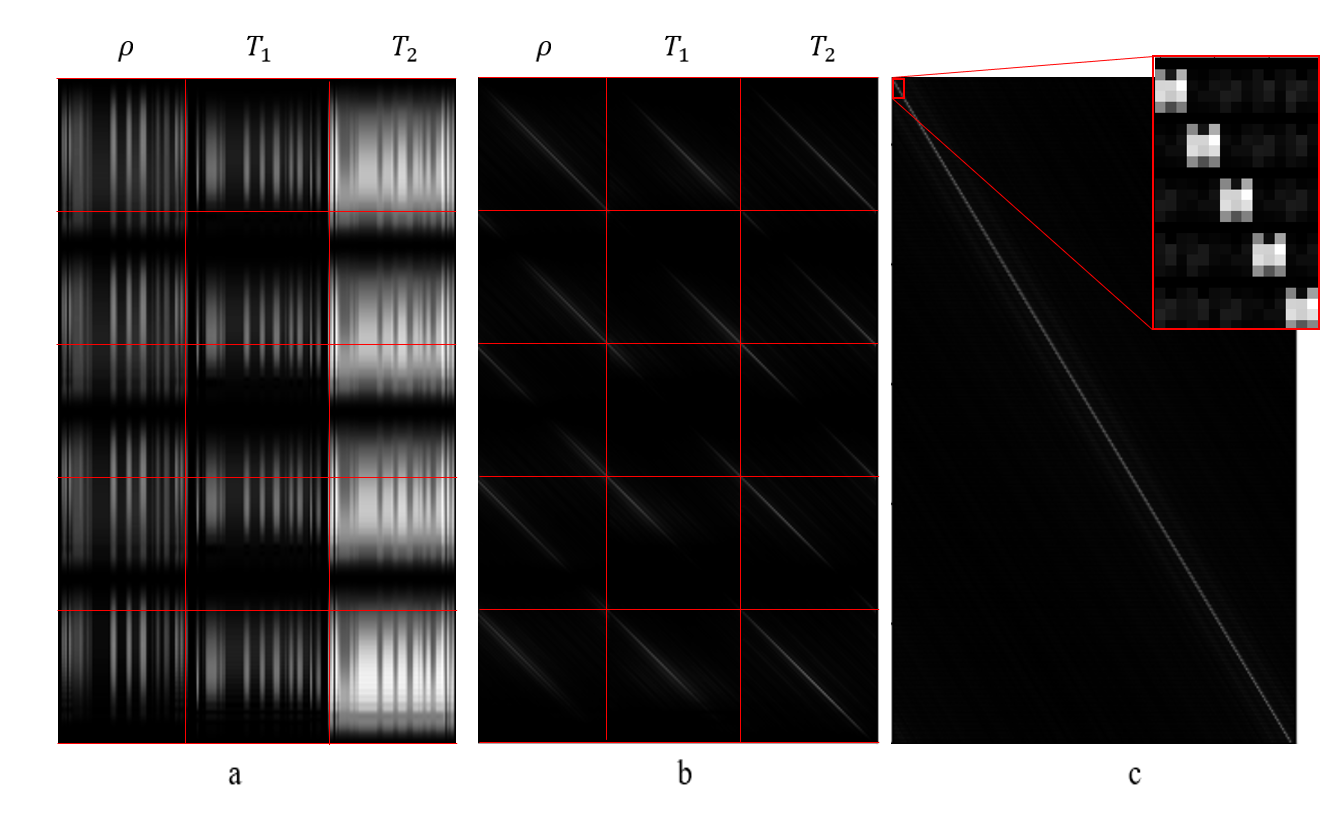
Figure 1:
Graphical representation of a portion of
the Jacobian (1120 rows times 672 columns). The red lines separate different
block corresponding to the three tissue properties and the five sets of
phase-encodings. The Out-of-sync sequence (fig. 2) is taken as an example. (a)
magnitude of $$$J$$$, (b)
magnitude of $$$JF$$$, obtained
by row-wise Fourier transform. Observe that $$$JF$$$ has diagonally-dominant blocks, while $$$J$$$ does not. (c) magnitude of $$$JF$$$,
re-arranged. In this representation, the diagonal blocks of size $$$N_i \times 3$$$ are clearly dominant.
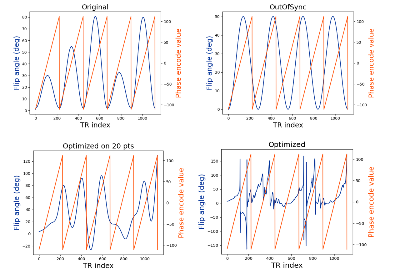
Figure 2: Flip-angle sequence (blue) and phase-encode values
(orange) for the four evaluated sequences
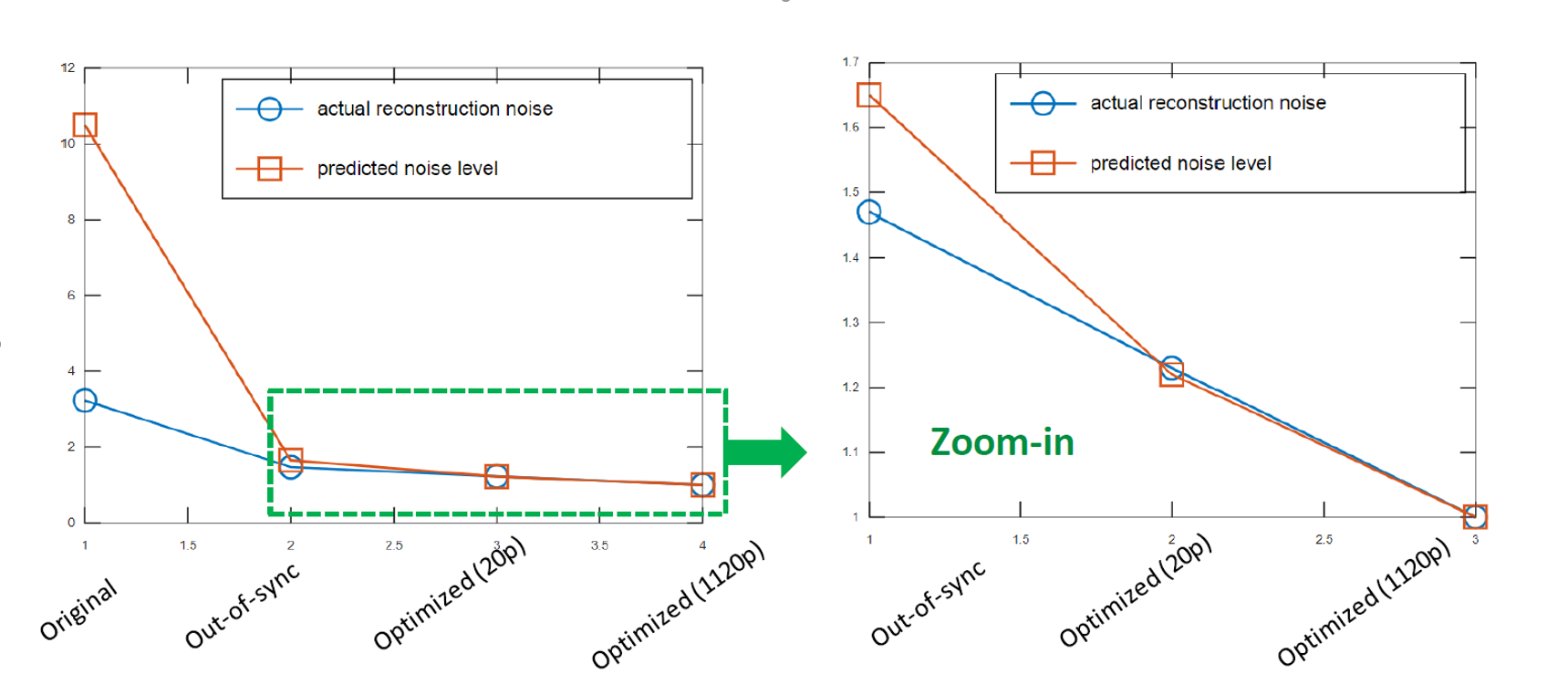
Figure 3: Correspondence between BLAKJac estimates and actual
noise deviations from reconstruction results. Even if the two curves do not quantitatively agree, they do display the same decreasing trend.
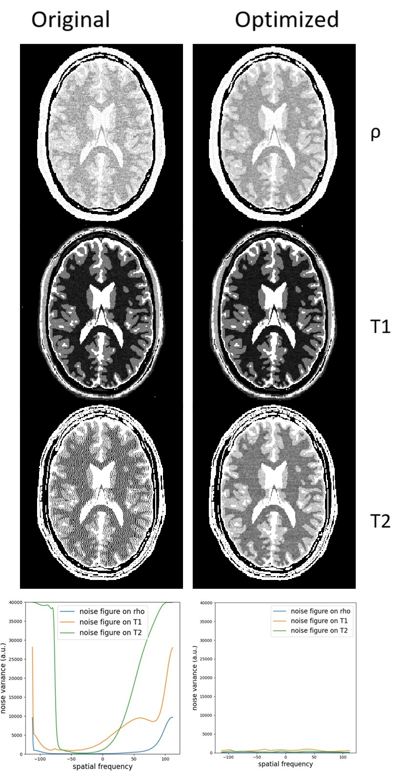
Figure 4: Reconstructed parameter maps and BLAKJac-estimated
frequency-domain plots of variances of the noise (bottom row); left: Original sequence;
right: Optimized sequence. In the images, narrow windowing has been applied to
visualize the noise. Vertical axis of the graphs is the noise variance,
arbitrary units, but same scale between the two graphs. The graphs show the
noise-enhancement for the high phase-encoding values in the Original sequence,
which is seen in image as high-spatial-frequency noise in the corresponding
images.
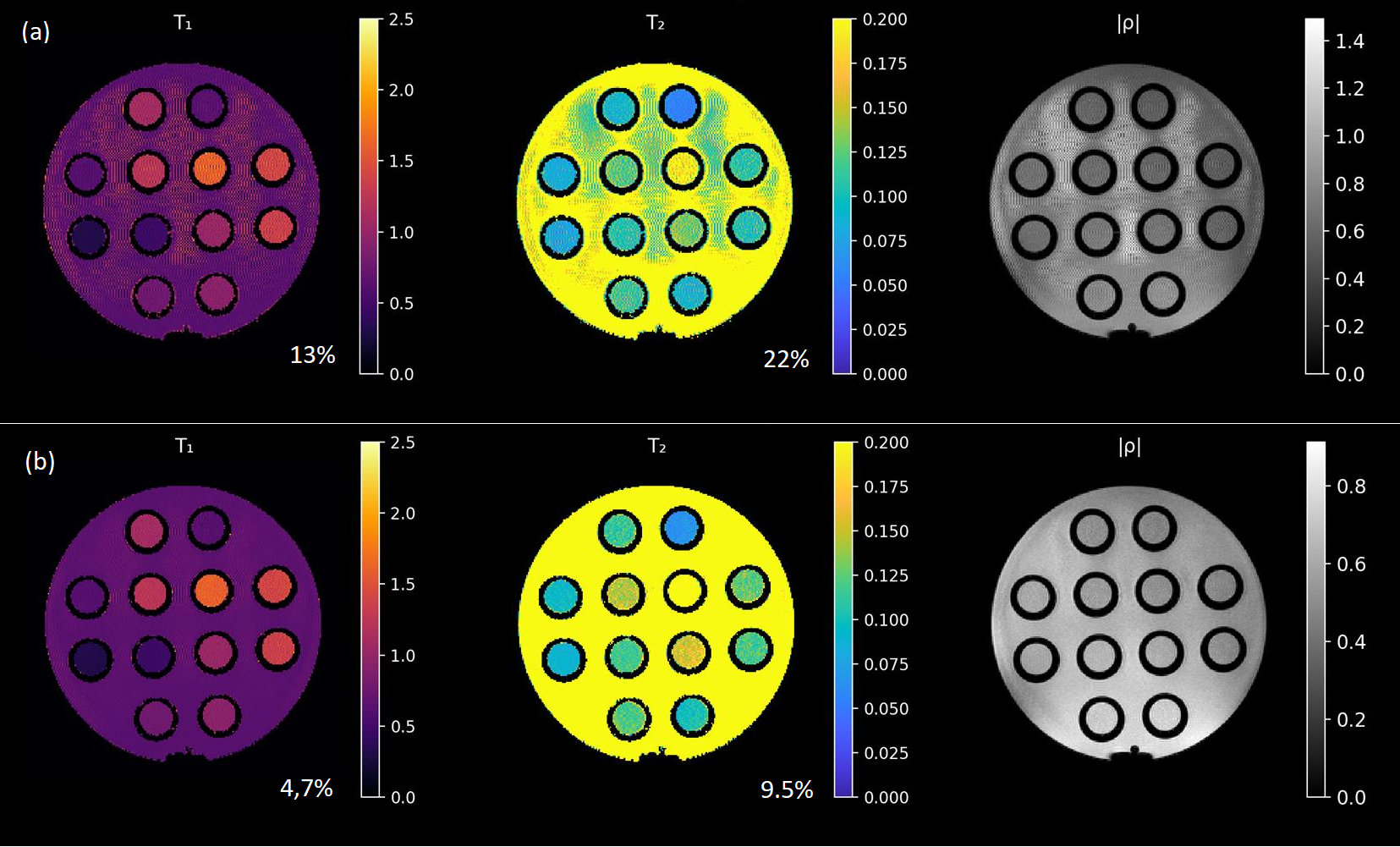
Figure 5: The
suppression of the
high-spatial frequency noise in (a) is readily apparent in the maps
in (b), confirming the prediction of the BLAKJac analysis. The figures indicate the relative noise standard deviation value, averaged over the 12 vials.