2994
Few-shot deep learning for kidney segmentation1Radiology, UT southwestern medical center, Dallas, TX, United States
Synopsis
MR kidney image segmentation is an important enabler of radiomics analysis and assessment of kidney size, morphology and renal disease. Deep learning methods are state-of-the-art techniques for segmentation. Training of a robust model with high accuracy requires a large dataset. Manually drawing masks is time-consuming and labor-intensive for a large number of datasets. Furthermore, different masks are required in training for different MR modalities. In this study, we investigated the feasibility of kidney segmentation using deep learning models trained with MR images from only a few subjects. We tested the hypothesis that few-shot deep learning may achieve accurate kidney segmentation.
Introduction
Segmentation is an essential step in radiomics analysis of renal disease on MRI images 1 . Deep convolutional neural networks (CNNs) are state-of-the-art techniques to perform segmentation in medical imaging 2, 3. Training of a robust CNN model requires a large amount of data including images and ground truth masks. However, creating such masks is very costly and time consuming. The problem intensifies especially for body MRI. Ground truth masks have to be drawn for each image acquisition (i.e. MR sequence) since motion prevents from transferring ground truth masks among different sequences. The shortages of ground truth data are more frequent scenarios in clinical applications of deep learning segmentation. To overcome this problem, few-shot deep learning, one specific type of weakly supervised learning, has been proposed to learn from a limited number of examples with supervised information 4, 5. In this study, we investigated the feasibility of kidney segmentation using CNN models trained with a few sets of MRI images. We tested the hypothesis that few-shot deep learning may achieve accurate kidney segmentation by fully utilizing 3D features of MRI images in data augmentation.Methods
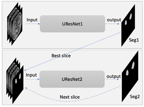
T1-weighted (T1w) MR images and kidney masks were downloaded from the website of the Combined (CT-MR) Healthy Abdominal Organ Segmentation (CHAOS) challenge 6. A total of 20 sets of MR T1w out-phase images and kidney masks were used to train and test CNN models for few-shot kidney segmentation in this study. The effective slice thicknesses including slice spacing varied between 5.5-9.5 mm and the number of slices for each subject was between 26 and 50.In this study, transformations for data augmentation included 3D rotation (x765), 3D radial distortion (x2), 2D shear deformation (x3), denoising or adding noise to images (x2-6), and intensity inversion (x2). The total number of data augmentation transformations varied from 9,180 to 55,080 depending on the number of selected subjects. The proposed CNN model is a cascaded network including two 2D Unet models shown in Fig. 1 3. The Unet architecture with a backbone of ResNet34 was used 7. Unet models based on TensorFlow were downloaded from github (https://github.com/qubvel/segmentation_models). The Unets were trained for three scenarios: 1. One subject with a slice thickness of 5.5 mm with augmentations (N=55,080); 2. Three subjects with augmentations (N=18,360); 3. Six subjects (randomly selected half of images) with augmentation (N=9,180). Total number of data augmentations, including the number of subjects, was kept similar (N=55,080) for the three above-mentioned scenarios. Dice coefficients were calculated to compare between the ground truth masks and the predicted masks.
Results
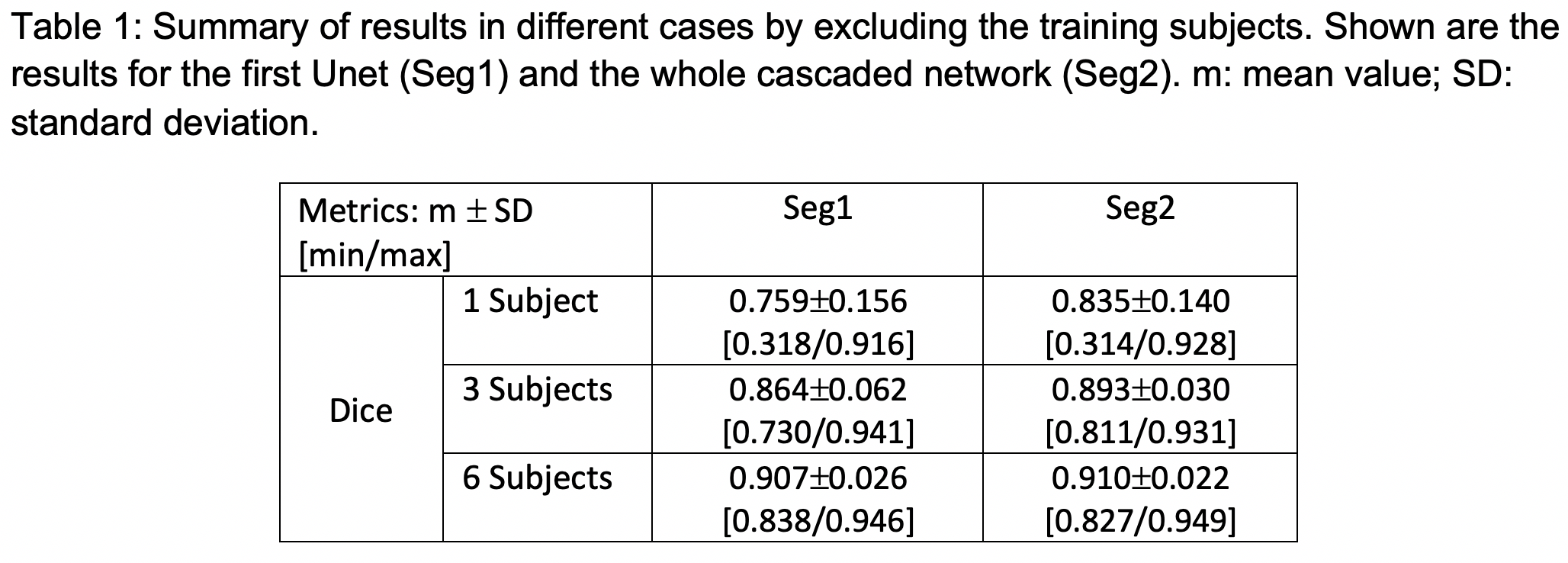
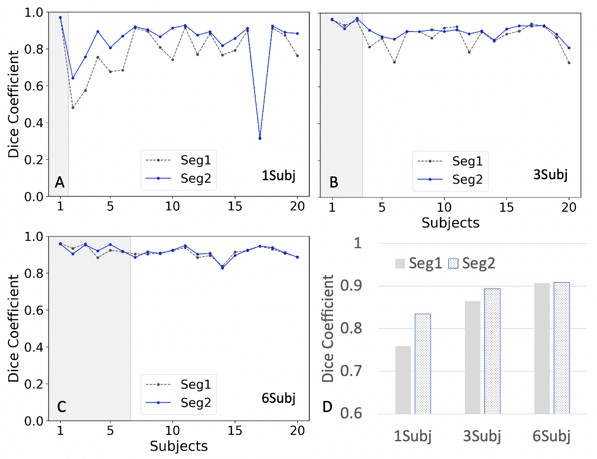
Fig. 2 shows the plots of Dice coefficients of Seg1 and Seg2 using different number of training subjects. Fig. 2a shows the results from the model trained using only a single subject. Dice coefficients were close to 0.8 for the most of 19 testing subjects except a few subjects with dramatically different contrast. However, the segmentation results in Fig. 2b were dramatically improved by adding two more subjects to the training set: one with a large portion of perirenal fat and one with post-contrast images. Fig.2c shows that the segmentation results were further improved by adding three additional subjects into the training set. The cascaded network (Seg2) exhibited substantial advantage over a single Unet (Seg1) when using a single training subject. This advantage disappeared when using six training subjects. Table 1 summarizes the Dice coefficients for the above cases.Discussion/Conclusion
Our few-shot segmentation approach obtained high accuracy with mean Dice coefficient of 0.91 using six training subjects. The best mean Dice coefficient of 0.91 using six training subjects is much higher than the previous reported Dice value of 0.78 for kidney trained using 36 subjects 8 and is close to the previous reported Dice coefficient of 0.96 for kidney from the model trained using 2000 subjects 9. The cascaded network help diminish the underfitting problem to some extent due to difference of image contrast and morphology. The underfitting issue was greatly reduced and even disappeared by adding more subjects with different contrasts.In conclusion, we demonstrate the feasibility of kidney segmentation using deep learning CNN models trained with only a few subjects. We found that the proposed few-shot deep learning approach obtained high-quality segmentation of kidney using T1w MR images. Our approach provides a solution to segmentation of kidneys in T1w imaging when the number of ground truth masks is limited.
Acknowledgements
This project is supported by NIH grants R01CA154475, U01CA207091, and P50CA196516.References
1. de Leon, A.D., P. Kapur, and I. Pedrosa, Radiomics in Kidney Cancer: MR Imaging. Magn Reson Imaging Clin N Am, 2019. 27(1): p. 1-13.
2. LeCun, Y., Y. Bengio, and G. Hinton, Deep learning. Nature, 2015. 521(7553): p. 436-44.
3. Ronneberger, O., P. Fischer, and T. Brox U-Net: Convolutional Networks for Biomedical Image Segmentation. arXiv e-prints, 2015. arXiv:1505.04597.
4. Li, F.F., R. Fergus, and P. Perona, One-shot learning of object categories. Ieee Transactions on Pattern Analysis and Machine Intelligence, 2006. 28(4): p. 594-611.
5. Zhou, Z.H., A brief introduction to weakly supervised learning. National Science Review, 2018. 5(1): p. 44-53.
6. Emre Kavur, A., et al. CHAOS Challenge -- Combined (CT-MR) Healthy Abdominal Organ Segmentation. 2020. arXiv:2001.06535.
7. He, K., et al. Deep Residual Learning for Image Recognition. 2015. arXiv:1512.03385.
8. Bobo, M.F., et al., Fully Convolutional Neural Networks Improve Abdominal Organ Segmentation. Proc SPIE Int Soc Opt Eng, 2018. 10574.
9. Kline, T.L., et al., Performance of an Artificial Multi-observer Deep Neural Network for Fully Automated Segmentation of Polycystic Kidneys. J Digit Imaging, 2017. 30(4): p. 442-448.
Figures