2979
A generalized magic angle effect model for better characterizing anisotropic T2W signals of human knee femoral cartilage
Yuxi Pang1
1Dept. of Radiology, University of Michigan, Ann Arbor, MI, United States
1Dept. of Radiology, University of Michigan, Ann Arbor, MI, United States
Synopsis
Collagen fibril microstructural distributions in articular cartilage are extremely complex. The simplistic two halves radially segmented cartilage in clinical T2W sagittal knee images may not truly represent histologically defined deep and superficial zones. Furthermore, the normal to femoral cartilage surface varies considerably within imaging slices from the lateral to medial side of knee. Consequently, the standard magic angle effect (MAE) functions become inadequate for characterizing the observed anisotropic T2W signals in knee cartilage. Thus, a generalized MAE model is presented for better quantifying anisotropic T2W signals in the clinical studies of human knee articular cartilage.
INTRODUCTION
Anisotropic transverse relaxation rate, $$$R_2^a(θ)$$$, reportedly possesses the best sensitivity in detecting cartilage early degenerations.1 Recently, an efficient $$$R_2^a(θ)$$$ measurement method has been developed, where an internal reference (REF) has to be deduced from T2W femoral cartilage sagittal images, based on the standard magic angle effect (sMAE) model.2 Unfortunately, the vast majority of imaging slices can not be adequately characterized due to complex collagen microstructural distributions and an irregular femoral cartilage surface. This work is thus to propose a generalized MAE (gMAE) model to better characterize anisotropic T2W signals in human knee cartilage.METHODS
(1) Theory: Relative to cartilage surface normal, collagen fibers are respectively in perpendicular, random and parallel orders in the superficial (SZ), transitional (TZ), and deep (DZ) zones.3-4 Water proton dipolar interactions within collagen fibers are on average along the fiber direction.5 Given a voxel comprising fibers distributed in an axially symmetric system (Figure 1A), the orientation dependence of $$$R_2^a(θ)$$$ can be derived by averaging an ensemble of dipolar interactions associated with differently orientated fibers. A representative fiber is shown (Figure 1A) forming angle $$$θ$$$ to $$$B_0$$$, and angle $$$α$$$ to cartilage surface normal ($$$\overrightarrow{n}$$$) that makes angle $$$ε$$$ with $$$B_0$$$. Note, $$$α$$$ and $$$ε$$$ are stationary but $$$φ$$$ (azimuthal angle) and $$$θ$$$ become spatial or time dependent.6 With spherical law of cosines (i.e. $$$\cos\theta=\cos\alpha\cos\epsilon+\sin\alpha\sin\epsilon\cosφ$$$) and after an average over $$$φ$$$ from 0 to 2π, the function $$$⟨(3cos^2θ-1)^2⟩$$$ can be expressed by Eq. 1, here called the gMAE function.$$f(α,ε)=(1/4)(3cos^2α-1)^2 (3cos^2ε-1)^2+(9/8)(sin^4α sin^4ε+sin^22αsin^22ε) \; (1) $$When $$$α$$$=0° and 90°, $$$f(α,ε)$$$ returns respectively to the standard MAE (sMAE) functions of $$$(3cos^2ε-1)^2$$$ and $$$1-3sin^2ε+(27⁄8)sin^4ε$$$ for collagen fibers in the DZ and SZ.4 (2) T2W MR imaging: T2W sagittal images were acquired from an asymptomatic knee of one consented subject at 3T, using an interleaved MSME (n=8) TSE sequence and a 16-channel T/R knee coil. Key parameters were listed here: FOV = 128*128*96 mm3; voxel size = 0.6*0.6*3.0 mm3; Compressed SENSE factor = 2.5; TR = 2500 ms; scan time =7.42 minutes. Only T2W images with TE=48.8 ms were evaluated. A high-resolution 3D image of the same knee was also acquired (Figure 2). (3) Modeling MAE in T2W: Femoral cartilage was segmented angularly and radially following an established protocol2, average signal intensities ($$$S$$$) from segmented ROIs can be expressed by Eq. 2, $$S=S_0exp\{-(R_2^i+R_2^a*f(α,ε))TE\} \;(2) $$ where $$$S_0, R_2^i, R_2^a$$$ and $$$TE$$$ represent respectively initial signal ($$$TE$$$=0), isotropic and anisotropic $$$R_2$$$, and echo time. In a logarithmic scale, Eq. 2 was fitted to segmented ROIs, i.e. $$$y(ε)=A-B*f(α,ε)$$$. An independent variable was $$$ε$$$ and three model parameters were $$$A=(Log S_0-R_2^i TE)$$$, called an REF2; $$$B=R_2^a*TE$$$ and $$$α$$$. For comparison, the fitting using Eq. 2 was named “Fit A” for both the DZ and SZ data, whereas the fittings were called “Fit B” with $$$α$$$=0 for the DZ data, and “Fit C” with $$$α$$$=90° for the SZ data. Goodness of fit was measured by the root-mean-square error (RMSE), and statistical significant differences were assessed by an F-test, with significance indicated by P < .05. All data analysis was performed with in-house software written in IDL 8.5.RESULTS AND DISCUSSION
Figures 1B-D present respectively four $$$f(α,ε)$$$ profiles with $$$α$$$=0° (red), 33°(green), 57° (blue) and 90° (black) (B), two schematic sagittal imaging slices with surface normal vectors $$$\overrightarrow{n}$$$ (red) and $$$\overrightarrow{m}$$$ (green) making an angle $$$α$$$ (C), and the spatial distribution of $$$f(α,ε)$$$ when considering a spherical femoral cartilage containing 11 different fibril microstructural distributions from the innermost ($$$α$$$=0°) to outermost ($$$α$$$=90°) layers. Because of $$$f(α,ε)$$$ symmetry, e.g. $$$f(α,0)$$$=$$$f(0,α)$$$, $$$α$$$ can be interpreted either as the spread of fiber directions around a preferential orientation axis (i.e. $$$\overrightarrow{n}$$$) or as the deviation of an orientation axis from $$$B_0$$$ (i.e. $$$\overrightarrow{m}$$$ ) when $$$ε$$$=0°.Figure 2A highlights the curved femoral cartilage surface in a volume-rendered knee image, and Figure 2B pinpoints the spatial locations on a coronal image of six T2W sagittal imaging slices, i.e. S13, S09, and S05 from medial side (Figures 3A-C) and S29, S25, and S20 from lateral side (Figures 4A-C). Clearly, Fit A provided significantly (P<.01) better fits for the edged imaging slices when compared with Fit B or Fit C, for instance, for Slice 05 (Figure 3A) and Slice 29 (Figure 4C) in the DZ, and Slice 20 (Figure 4A) in the SZ, signifying a curved surface in consistence with theoretical predictions.
Overall, Fit A significantly outperformed Fit B (Figure 5A) in the DZ (0.239±0.122 vs. 0.267±0.097, P=.014) and Fit C (Figure 5B) in the SZ (0.183±0.081 vs. 0.254±0.085, P<.001). A relatively smaller average angle $$$α$$$ was observed in the DZ when compared to that in the SZ, i.e. 38.5±34.6° vs. 45.1±30.1°, P<.43, in good agreement with the reported fibril microstructural arrangements. Moreover, an REF was significantly larger when using Fit A (red solid line) in both the DZ (Figure 5C) and the SZ (Figure 5D).
These comparison results demonstrate that the proposed gMAE function could not only better characterize anisotropic T2W signals in femoral cartilage but it also provides an REF from both the DZ and SZ cartilage.
CONCLUSION
The proposed generalized MAE model is demonstrated for better characterizing anisotropic T2W signals in the human knee femoral cartilage.Acknowledgements
This work was in part supported by the Eunice Kennedy Shriver National Institute of Child Health & Human Development of the National Institutes of Health (NIH) under Award Number R01HD093626 (to Prof. Riann Palmieri-Smith).References
- Hanninen N, Rautiainen J, Rieppo L, Saarakkala S, Nissi MJ. Orientation anisotropy of quantitative MRI relaxation parameters in ordered tissue. Sci Rep 2017;7(1):9606.
- Pang Y, Palmieri-Smith RM, Malyarenko DI, Swanson SD, Chenevert TL. A unique anisotropic R2 of collagen degeneration (ARCADE) mapping as an efficient alternative to composite relaxation metric (R2 -R1 rho ) in human knee cartilage study. Magn Reson Med 2019;81(6):3763-3774.
- Xia Y. Magic-angle effect in magnetic resonance imaging of articular cartilage: a review. Invest Radiol 2000;35(10):602-621.
- Grunder W. MRI assessment of cartilage ultrastructure. NMR Biomed 2006;19(7):855-876.
- Berendsen HJC. Nuclear magnetic resonance study of collagen hydration. J Chem Phys 1962;36(12):3297-3305.
- Hennel JW, Klinowski J. Magic-angle spinning: a historical perspective. New techniques in solid-state NMR: Springer; 2005. p 1-14.
Figures
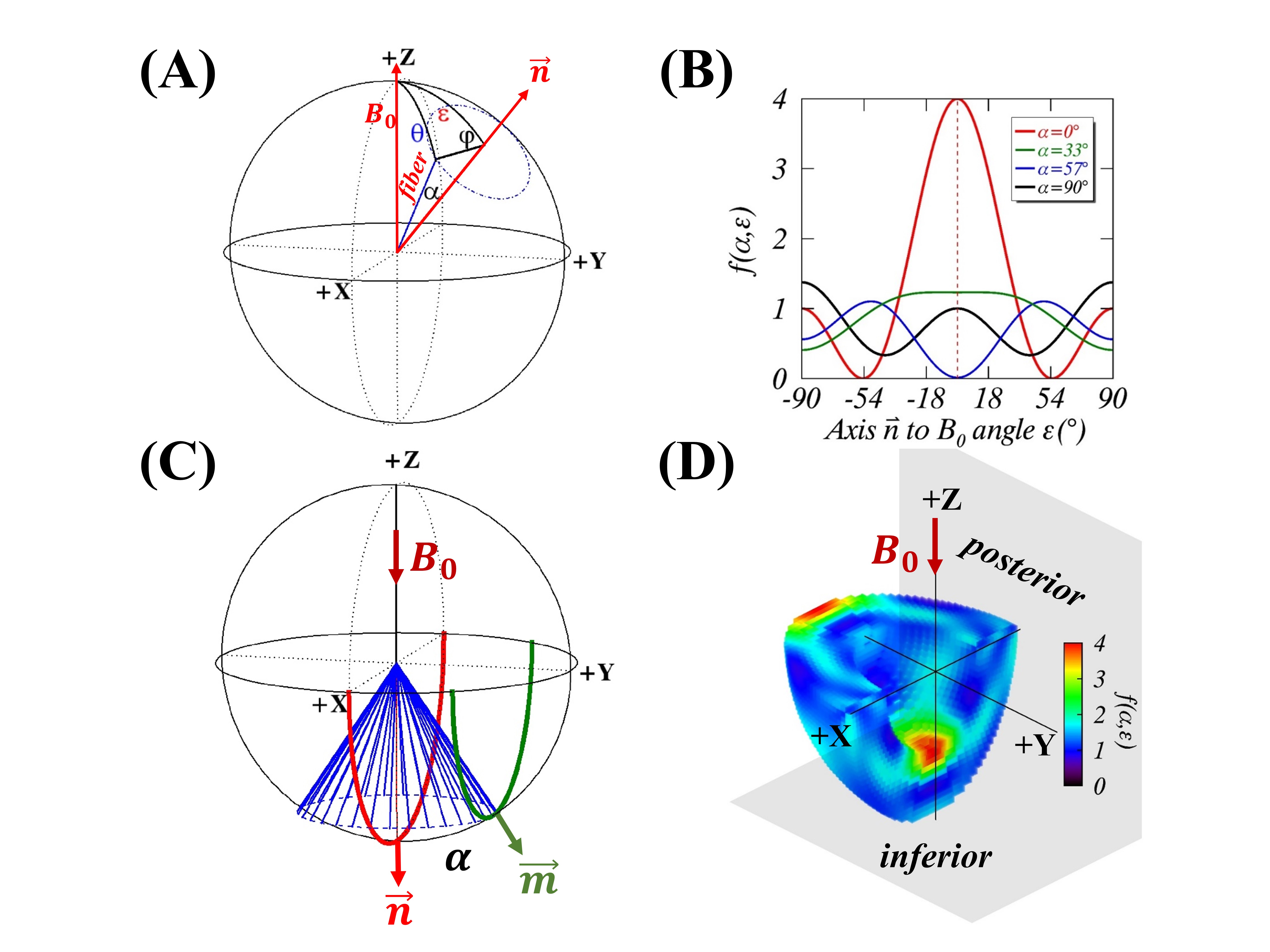
FIGURE 1. An axially symmetric model for collagen fibril distributions (A), and four representative $$$f(α,ε)$$$ profiles (B). Two hypothetical
sagittal (XZ plane) imaging slices with femoral cartilage normal vectors, $$$\overrightarrow{n}$$$ and $$$\overrightarrow{m}$$$, making an angle of $$$α$$$ when $$$ε$$$=0° (C). Simulated $$$f(α,ε)$$$ of an assumed spherical femoral cartilage containing 11 different collagen fibril distributions from the innermost ($$$α$$$=0°) to outermost ($$$α$$$=90°) layers (D).
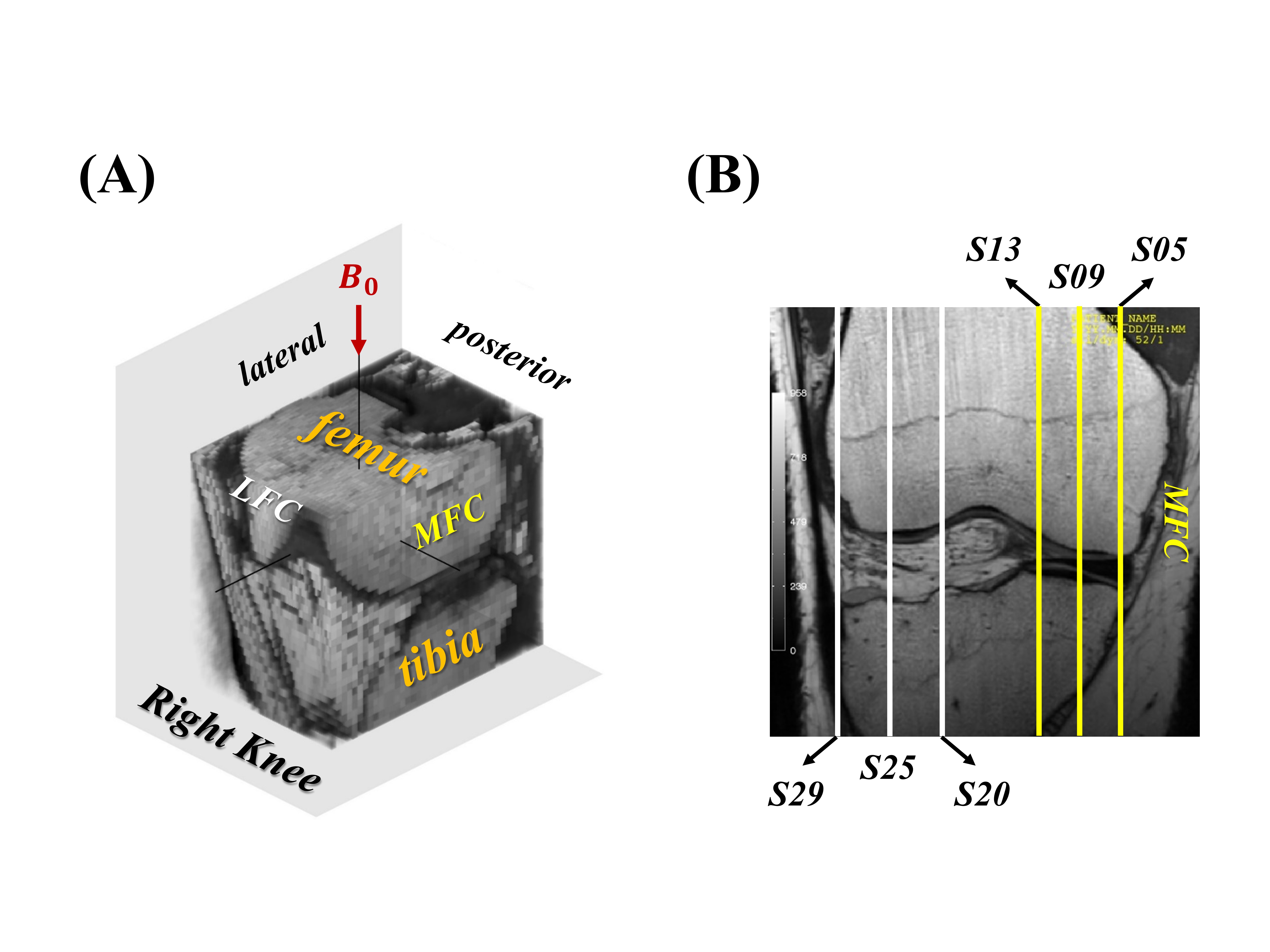
FIGURE 2. A volume-rendered high-resolution 3D right knee
image (A) and a coronal image (B) showing the locations of three sagittal slices (white lines) from lateral femoral condyle and of three sagittal slices (yellow lines) from medial femoral condyle .
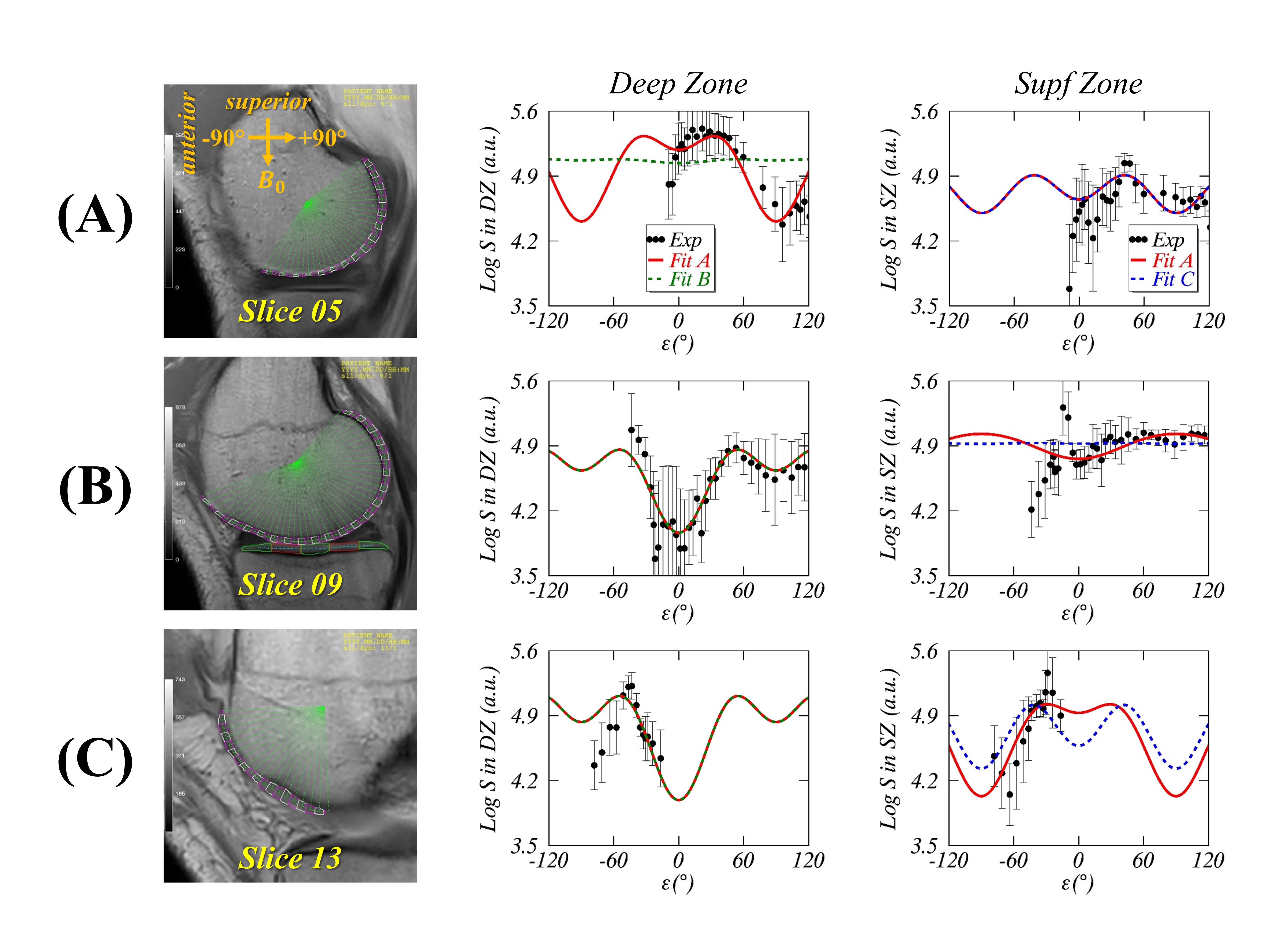
FIGURE 3. Three imaging Slices 05 (A), 09 (B) and 13 (C) from medial knee cartilage (the 1st column), superimposed
with segmented ROIs, from which the measured (black circles) average T2W
signal intensities were modeled using Fit A (solid red lines) and Fit B (dashed
green lines) in the deep zone (the 2nd column), and using Fit A and
Fit C (dashed blue lines) in the superficial zone (the 3rd column).
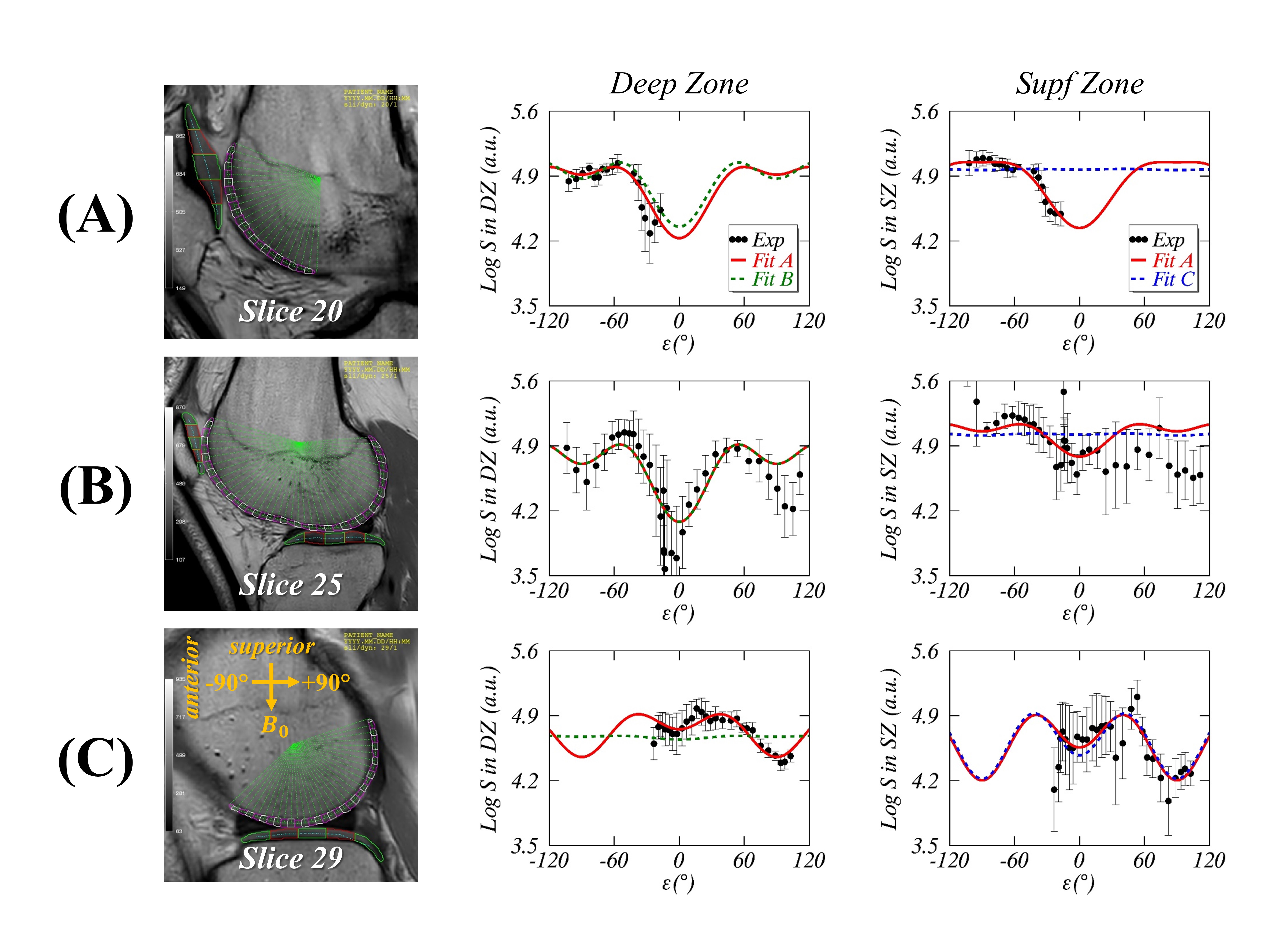
FIGURE 4. Three imaging Slices 20 (A), 25 (B) and 29 (C) from lateral knee cartilage (the 1st column), superimposed
with segmented ROIs, from which the measured (black circles) average T2W
signal intensities were modeled using Fit A (solid red lines) and Fit B (dashed
green lines) in the deep zone (the 2nd column), and using Fit A and
Fit C (dashed blue lines) in the superficial zone (the 3rd column).
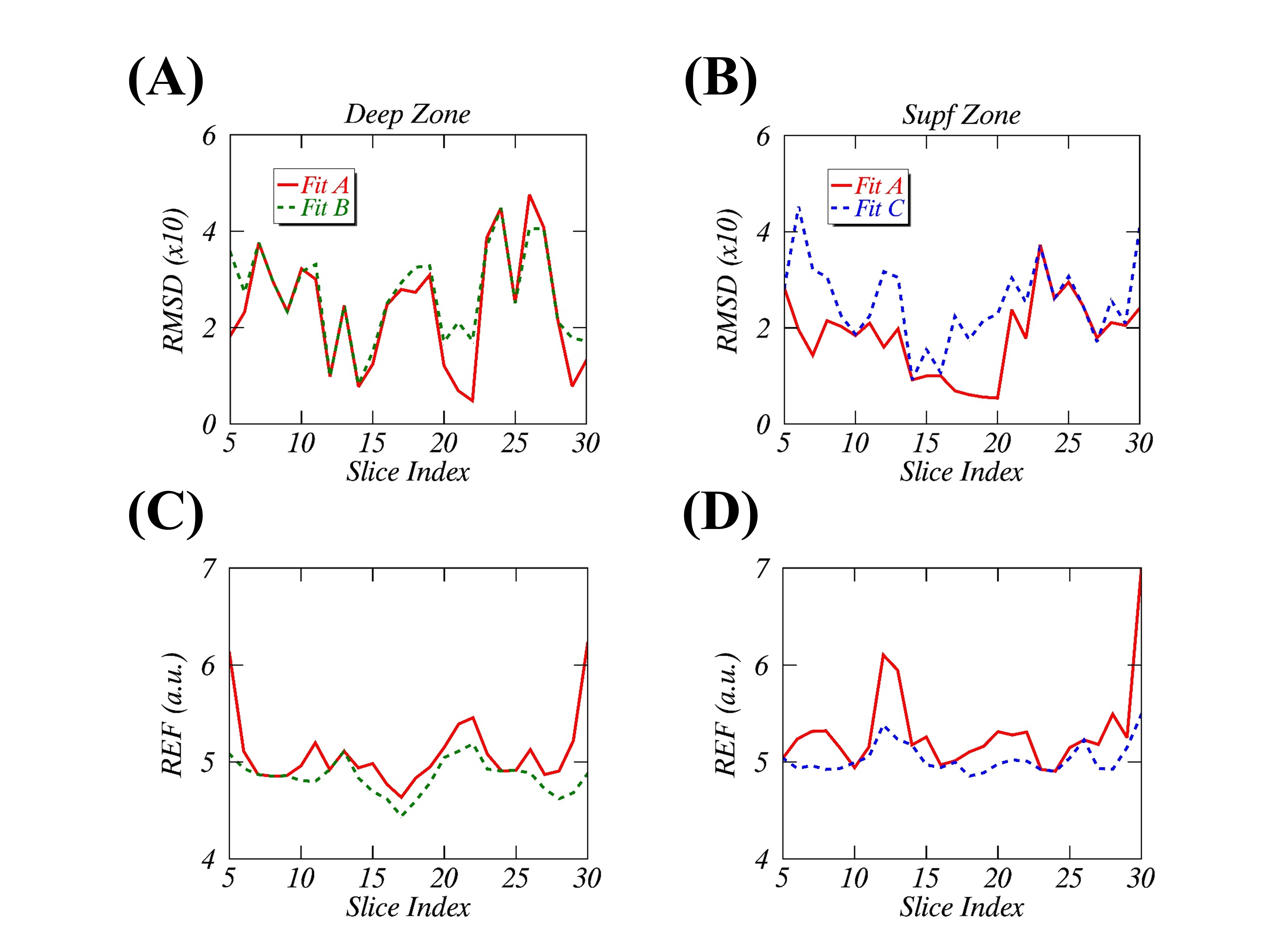
FIGURE 5. Comparisons of the root-mean-square deviations (RMSDs in A and B) and the fitted model parameter A (REFs in C and D) between using Fit
A (solid red lines) and using Fit B (dashed green lines) in the deep zone
(A and C) and between using Fit A and using Fit C (dashed blue lines)
in the superficial zone (B and D) for all imaging slices.