2978
Quantitative Magnetization Transfer in the Knee Meniscus: Minimizing Data Collection Protocols
Fatemeh Mostafavi1, Lumeng Cui1, Brennan Berryman2, Ives R. Levesque3, and Emily J. McWalter1,2
1Division of Biomedical Engineering, University of Saskatchewan, Saskatoon, SK, Canada, 2Department of Mechanical Engineering, University of Saskatchewan, Saskatoon, SK, Canada, 3McGill University, Montreal, QC, Canada
1Division of Biomedical Engineering, University of Saskatchewan, Saskatoon, SK, Canada, 2Department of Mechanical Engineering, University of Saskatchewan, Saskatoon, SK, Canada, 3McGill University, Montreal, QC, Canada
Synopsis
A major challenge in the use of quantitative magnetization transfer (qMT) is the long scan time. One method to reduce scan time is acquiring fewer MT-weighted images. qMT mapping of the meniscus was performed in six cadaver knees. Fitting was repeated after systematically decreasing the number of input scans and comparing the results to a reference dataset (10 MT-weighted images). A set of eight MT-weighted images fit to a two-pool model with Gaussian lineshape was found to have an acceptable level of agreement (a priori of 10%) with the reference dataset, saving approximately 8 minutes in scan time.
Introduction
The meniscus is an important tissue for knee joint function, but with disease its macromolecular structure breaks down. Quantitative magnetization transfer (qMT) has the potential to assess this breakdown because it probes the free protons (water) and bound protons (attached to macromolecules) within the tissue. qMT has been used successfully in articular cartilage and shows moderate correlations with biomechanical content and osteoarthritis1,2, although qMT work in the meniscus has been limited. However, qMT requires long scan sessions (up to an hour for one knee), which hinders its potential use in in vivo research studies. This study aims to determine how reducing the number of images used for parameter fitting affects the qMT outcome metrics, specifically, the T1 relaxation time of free pool (T1f), the T2 relaxation time of free pool (T2f) and restricted pool (T2b), the restricted pool fraction (f), and exchange rate (kf).Methods
Six cadaver knee specimens (3 males, mean age 70.3±9.3) were scanned at 3 T (MAGNETOM Skyra, Siemens, Erlangen, Germany). An in-house qMT-spoiled gradient-recalled echo (SPGR) based protocol was used to collect 10 MT-SPGR scans with off-resonance pulses (MT pulse power of 142, 426° and offset frequencies of 433, 1087, 2732, 6862, and 17235 Hz), one SPGR (no MT) scan, B1 (double angle method3) and T1 (variable flip angle method4) maps. The SPGR scans had the following parameters: field of view =160x160mm2, TR/TE=48/3ms, matrix=256x256, and slice thickness=3mm. The total scan time was approximately 1 hour. qMT parameters were estimated using a two-pool model fit with T1 of the bound pool fixed at 1s for both Gaussian and Super-Lorentzian lineshapes5-7. B1 maps were used for correction, and T1 maps were used for modelling; B0 correction was not included because of the small variation across the meniscus. These data were considered the reference dataset (Table 1). The data used for qMT fitting were then reduced systematically. An optimization scheme was not employed; instead, we examined all potential combinations for nine, eight, seven and six data point fits. For the purpose of this abstract, we present eight reduced datasets that showed promising results as assessed by the accuracy with respect to the reference standard (five designs with eight, two designs with seven, and one design with six MT-SPGR scans) (Table 2). Accuracy was expressed as the mean absolute percentage difference from the reference standard, and a Bland-Altman test was used to assess limits of agreement (LOA) set to 10% a priori8.Results
qMT parameter maps showed reasonable results for the meniscus with r2=0.91±0.03 and r2=0.89±0.03 for the Gaussian and Super-Lorentzian fits, respectively (Figure 1). Overall, parameters from fits using the Gaussian lineshape was less sensitive to a reduction in data than the Super-Lorentzian lineshape (Figure 2). Reduced datasets #4, #5, #6, and #8 showed a mean absolute percentage difference of more than 10% for some parameters and are therefore not suitable candidates. This was most evident for kf and T2b. For the Bland-Altman LOA analysis, the Gaussian lineshape fit using design #3 performed best with a 95% confidence interval (CI) of LOA < 10% for all parameters except kf and LOA < 10% for all parameters (Figure3). A proportional bias was found in the Bland-Altman plot of f for design #3 (p < 0.05), however, the equity line was within the 95% CI of the mean differences indicating the bias is not significant. For the Super-Lorentzian lineshape, no design showed adequate agreement for all parameters (95% CI of LOA <= 10 %).Discussion
Our results show differences of less than 10% in the Gaussian fit for design #3 (8 MT-SPGR data points) as compared to our reference dataset (10 MT-SPGR data points); this yields a time savings of approximately eight minutes. Our results are not surprising given findings in the brain that suggest a minimum of 7 points are required9. The mean absolute percentage differences for Gaussian lineshape data reduction schemes were smaller than those of Super-Lorentzian lineshape, suggesting that Gaussian-based fitting schemes are less sensitive to data reduction. The results show that the mean absolute percentage difference in T1f is small (<2% in Gaussian and <5% in Super-Lorentzian). Differences in T2f, T2b and f are acceptable (<10% for the Gaussian fit). The maximum differences tended to be for kf for both fits, indicating that kf is particularly sensitive to fitting strategy and input data in the meniscus. This is not surprising given previous work in the brain showing kf to be the most noisy parameter9. Although some designs show mean absolute differences less than 10% with the Super-Lorentzian lineshape for all qMT parameters (design #1, #2, #3), they did not show an acceptable level of agreement in Bland-Altman analysis (LOA <= 10%). This study used a systematic approach of assessing data reduction; alternatively, we could have used a global optimization approach, which has been applied previously in the brain10,11. Optimization strategies may be useful for further studying qMT data reduction in the meniscus.Conclusion
This study shows that, if a 10% error is acceptable for the particular application, it is possible to calculate qMT parameters with fewer MT-weighted images using a Gaussian lineshape fit, which in turn reduces the scan time.Acknowledgements
The authors would like to acknowledge funding from The Arthritis Society Young Investigator Operation Grant, Natural Sciences and Engineering Research Council Discovery Grant, the Saskatchewan Health Research Foundation, MITACS Accelerate, Siemens Healthineers, and University of Saskatchewan Devolved Scholarship Program.References
1. Stikov N, Keenan KE, Pauly JM, et al. Cross‐relaxation imaging of human articular cartilage. Magnetic resonance in medicine. 2011 Sep;66(3):725-34.2. Sritanyaratana N, Samsonov A, Mossahebi P, et al. Cross-relaxation imaging of human patellar cartilage in vivo at 3.0 T. Osteoarthritis and cartilage. 2014 Oct 1;22(10):1568-76.
3. Insko EK, Bolinger L. Mapping of the radiofrequency field. Journal of magnetic resonance. Series A (Print). 1993;103(1):82-5.
4. Deoni SC, Peters TM, Rutt BK. High‐resolution T1 and T2 mapping of the brain in a clinically acceptable time with DESPOT1 and DESPOT2. Magnetic Resonance in Medicine: An Official Journal of the International Society for Magnetic Resonance in Medicine. 2005 Jan;53(1):237-41.
5. Simard M. Quantitative magnetization transfer evaluation of the knee joint in magnetic resonance imaging, Master of Science, McGill University, 2016
6. Ramani A, Dalton C, Miller DH, et al. Precise estimate of fundamental in-vivo MT parameters in human brain in clinically feasible times. Magnetic resonance imaging. 2002 Dec 1;20(10):721-31.
7. Sinclair CD, Samson RS, Thomas DL, et al. Quantitative magnetization transfer in in vivo healthy human skeletal muscle at 3 T. Magnetic resonance in medicine. 2010 Dec;64(6):1739-48.
8. Giavarina D. Lessons in biostatistics. Biochem Medica. 2015;25:141-51.
9. Levesque IR, Sled JG, Pike GB. Iterative optimization method for design of quantitative magnetization transfer imaging experiments. Magnetic resonance in medicine. 2011 Sep;66(3):635-43.
10. Yarnykh VL. Fast macromolecular proton fraction mapping from a single off‐resonance magnetization transfer measurement. Magnetic resonance in medicine. 2012 Jul;68(1):166-78.
11. Cercignani M, Alexander DC. Optimal acquisition schemes for in vivo quantitative magnetization transfer MRI. Magnetic Resonance in Medicine: An Official Journal of the International Society for Magnetic Resonance in Medicine. 2006 Oct;56(4):803-10.
Figures
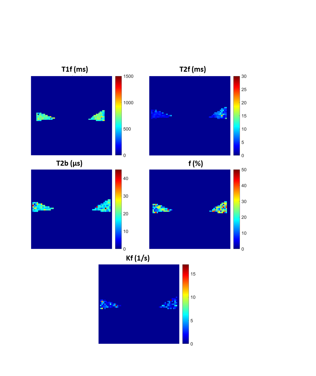
Figure 1: Representative
maps of QMT parameters in sagittal slice of specimen 1 using a Gaussian lineshape
fit.
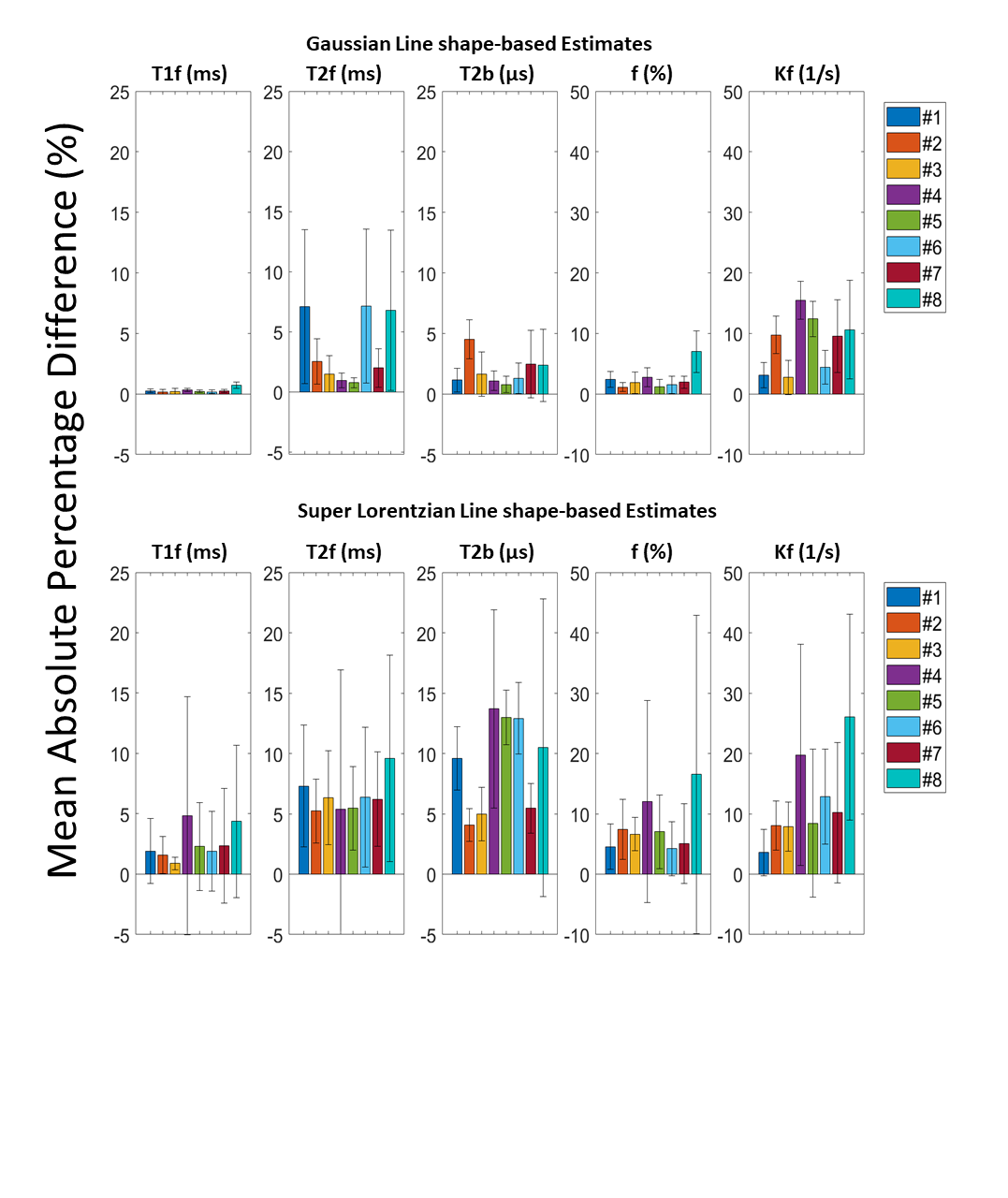
Figure 2: Mean absolute percentage difference from the
reference dataset for each design (1 through 8) for all qMT parameters (Top:
Gaussian, bottom: Super Lorentzian)
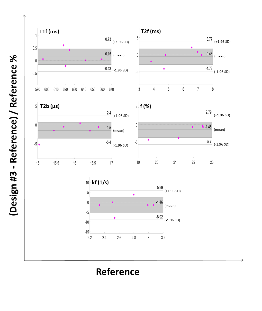
Figure 3: Reduction dataset #3 Bland Altman plots for each
qMT parameter. The shaded areas show the 95% confidence interval of mean
difference and the 1.96 SD lines show
the limits of agreement.
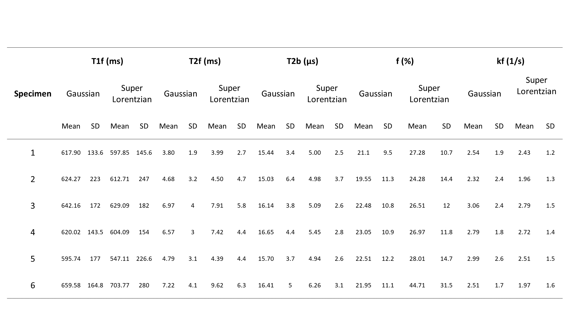
Table 1: qMT values for the meniscus reference dataset (based on 10 MT-SPGR scans)
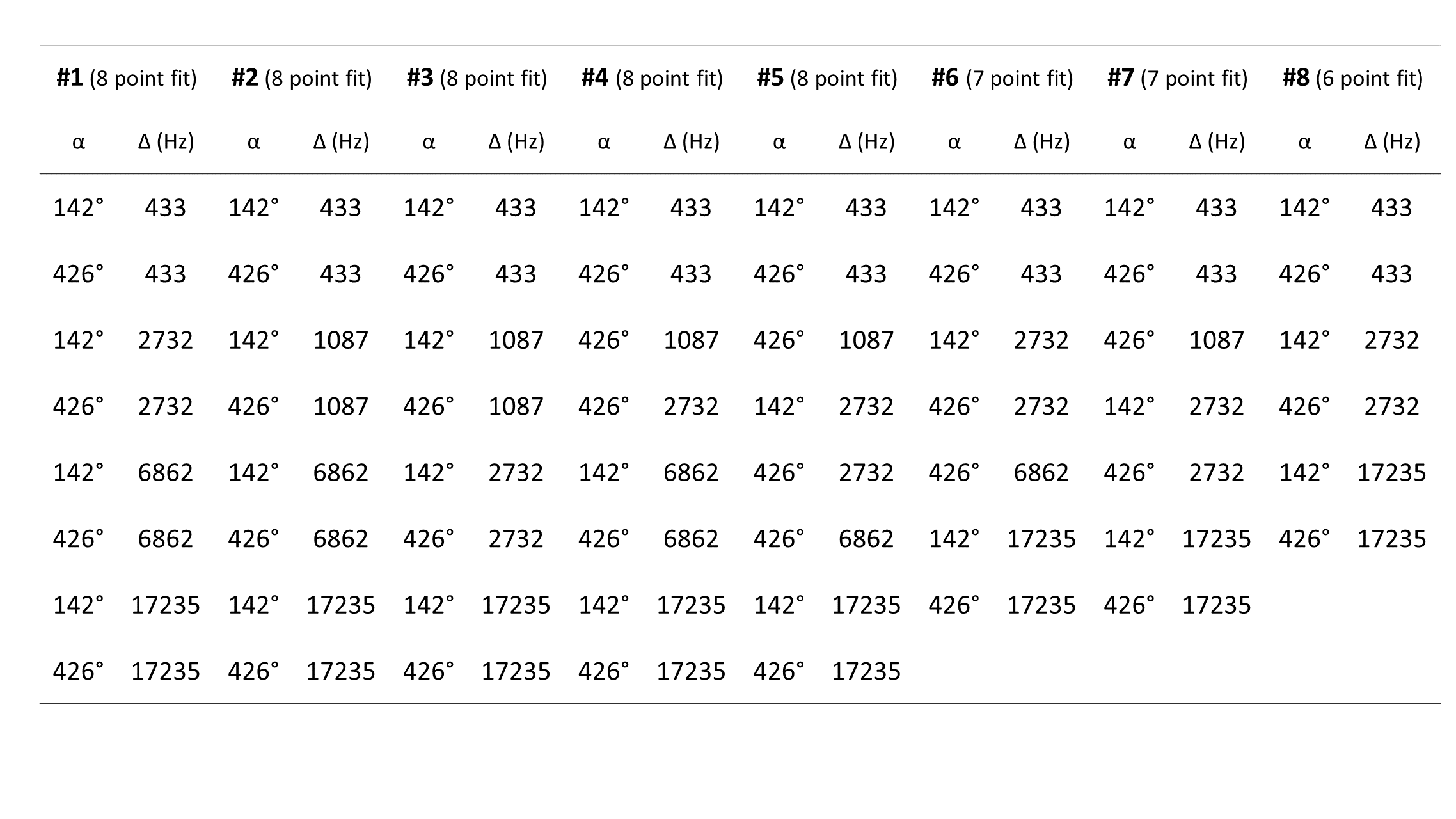
Table 2: MT-SPGR scans used for the reduced analysis. Eight different sets of input data
were compared. All datasets had different flip angles and offset frequencies.
Sampling sets #1 through #5 fit to 8 MT-SPGR scans; #6 and #7 fit to 7 MT-SPGR
scans; and #8 fit to 6MT-SPGR scans.