Introduction

Three-dimensional texture analysis of cartilage DESS images based on gray level co-occurrence matrices (GLCM) has previously demonstrated the ability to predict osteoarthritis (OA) onset years before manifestation of radiographic signs.¹ The prior study incorporated only a single set of fixed gray levels with 8-bin quantization and offset setting of 1. The aim of this study was to identify the optimal set of 3D Texture Analysis input parameters for classifying subjects that will develop OA. This was done by utilizing various machine learning protocols and using different gray level quantization ranges, numbers of bins, and offsets.

Methods

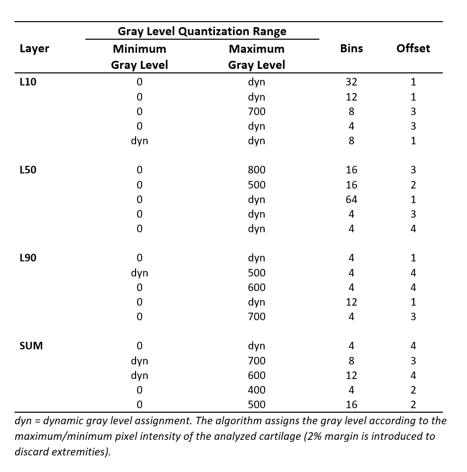
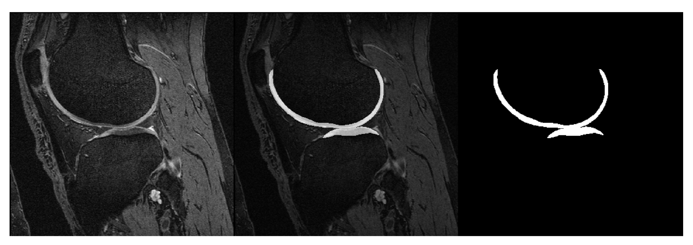
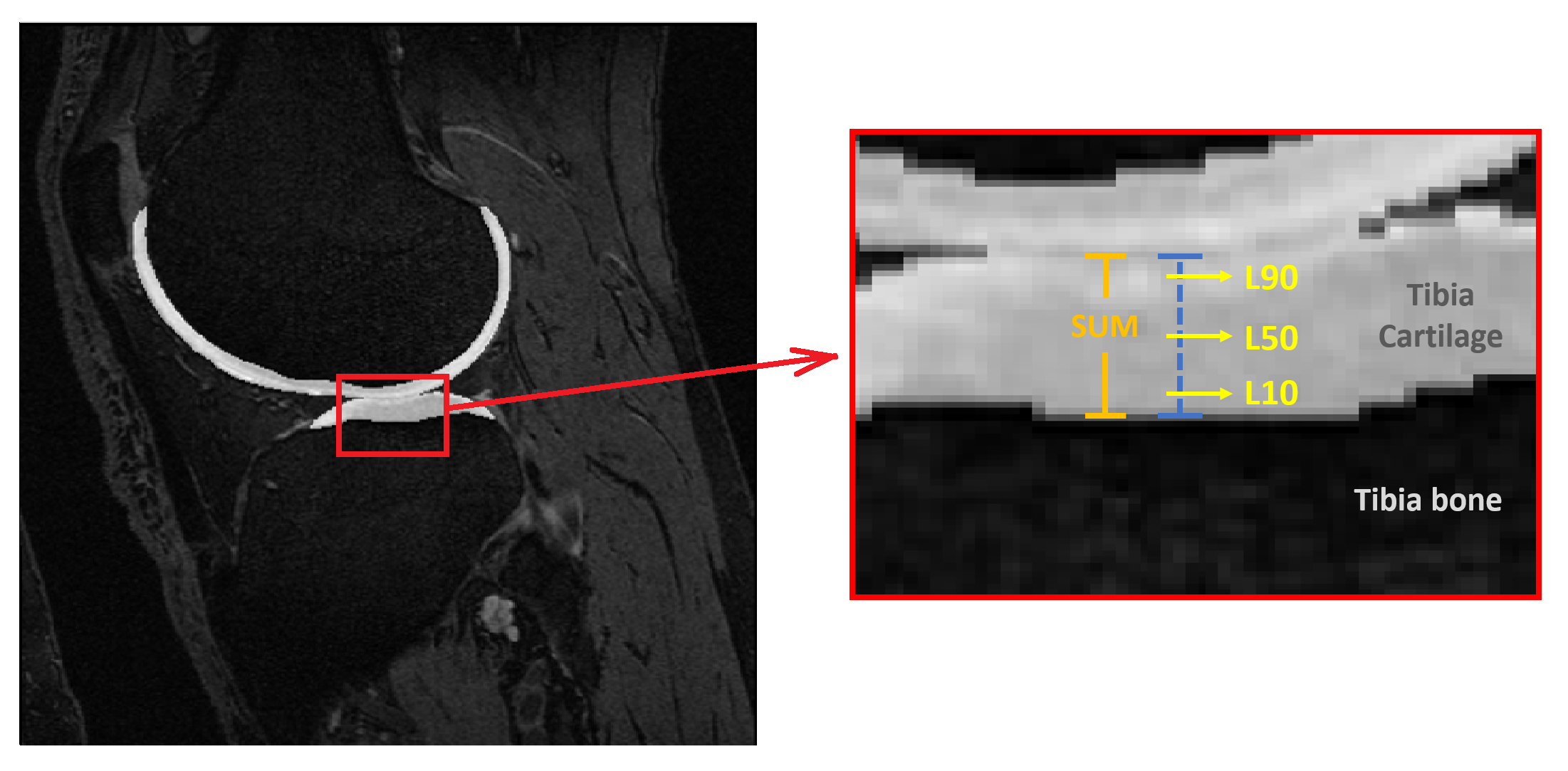
Baseline knee MRI of twenty subjects were obtained from the Osteoarthritis Initiative² (OAI) database. None of the selected subjects showed any radiographic signs of the disease at the baseline screening (Kellgren-Lawrence score, KL = 0). Ten control subjects were selected from the OAI Control cohort with KL = 0 at baseline and follow-up visits (CTRL group). Another 10 subjects were selected from the OAI Incidence or Progression cohort with rapid progression from KL = 0 at baseline to KL ≥ 2 at the 36-month visit (PRGS group). CTRL and PRGS groups were matched for sex, age (±2 years) and Body-Mass Index (BMI, ±2 kg/m2). For each subject the longitudinal relative BMI variation over 36 months was within 10%.

Femoral and tibial cartilages were automatically segmented from DESS images using a previously validated deep learning tool³ (Figure 1). Nineteen GLCM features were extracted for 4 different cartilage layers (Figure 2) at 10% (L10), 50% (L50) and 90% (L90) of the cartilage thickness, and SUM (full cartilage thickness). GLCMs were calculated using different gray level ranges with minimum and maximum levels assigned either statically or dynamically. The dynamic approach assigned gray levels according to the cartilage pixel intensity distribution with 2% margin to disregard outliers. Static maximum gray levels used were 300, 400, 500, 600, 700, 800. Pixel intensities outside the quantization range were included into the first or last bin. The used bin quantization schemes were 4, 8, 12, 16, 32 and 64 bins. Offsets of 1,2,3 and 4 were used.

Naïve Bayes (NB), Support Vector Machines (SVM, using radial basis function) and Multilayer Perceptron⁴ (MLP, 2 hidden layers, each containing 11 neurons) were trained and tested using all 19 features or selected features from either femoral or tibial cartilage. The training and testing were repeated 200 times to estimate the accuracy of each GLCM output feature set. The average accuracy across the 200 repetitions was calculated. Random initial conditions were assigned for each repetition as well as random training and testing split. The testing set consisted of either a single subject pair or 1-3 randomly selected subjects regardless of their cohort. The rest of the subjects were used for training. The training set was bootstrapped to always contain 20 subjects. Two hundred repetitions yielded one set of results for the chosen model.

Results

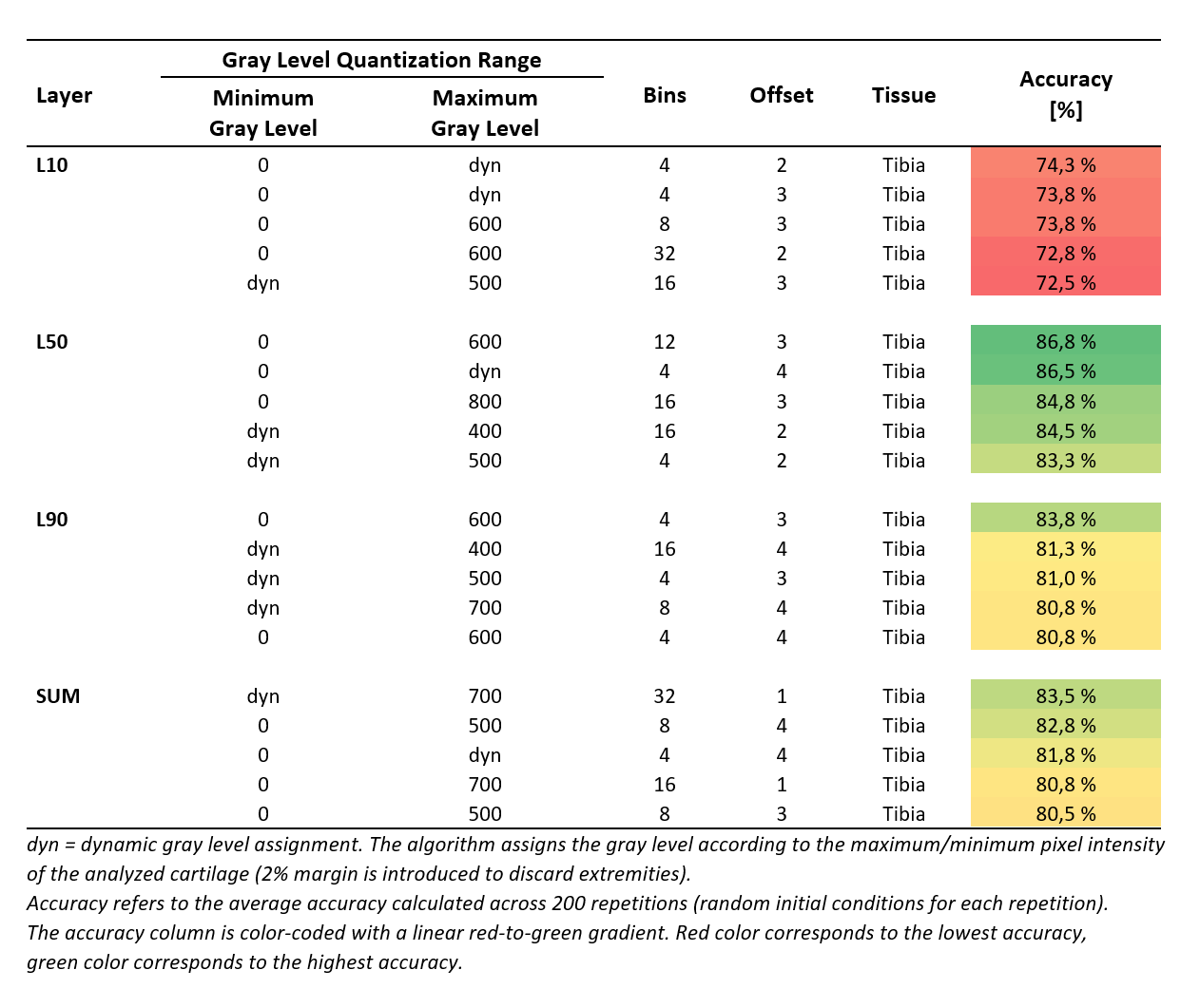
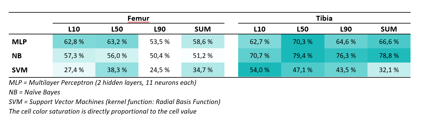
The highest accuracy (86.8%) was achieved using Naïve Bayes on tibial cartilage features (Table 1). The average difference between best and worst accuracies was 30.8 ± 11.2%. Using Naïve Bayes yielded the highest overall accuracy for tibial predictions (Table 2). Utilizing SVM yielded a performance spike (79.3%) with selected L50 tibial features, otherwise the accuracies for SVM predictions remained below 50%. Using MLP showed the highest overall accuracies in femoral L10 and L50 predictions (62.8% and 63.2% respectively). Best predictions were observed by using tibial L50 and SUM features. Tibial features outperformed femoral features across all models by 13.1% for L10; 16.2% for L50; 18.2% for L90; and 14.8% for SUM. A table of 5 best performers across all sets of results for each layer is presented (Table 3).

Discussion

The average difference between best and worst accuracies highlights the importance of the input parameter selection. Based on the results, dynamic gray level assignments and/or higher static maximum gray levels seem to benefit the prediction. The best accuracies were found to be associated with lower number of bins (4-12 bins seemed to be optimal with this subject dataset). Using Naïve Bayes provided the best results from tibia and using MLP seemed to be most beneficial for femoral features. SVM has shown good performance amongst OA studies found in the literature.⁵ This and the observed performance spike suggest that further parameter search with different kernel functions should be conducted.

The subject dataset in this study consisted of only 20 subjects and a single timepoint (baseline) due to the time-consuming nature and complexity involved with the 3D texture analysis. The small sample size might arguably be the biggest limitation of this study due to its probable impact on the classifiers. Future studies with larger sample sizes will be performed in order to build upon the findings of this study.

Conclusion

The GLCM features calculated with 3D Texture Analysis showed promising predictive capabilities. Adjusting the minimum and maximum gray levels to the analyzed cartilage had a positive impact on the predictions. Lower bin quantization numbers also displayed better accuracy. Using Naïve Bayes yielded the most convincing results. A further study is warranted to implement machine learning classification models and therefore maximize the predictive potential.

Acknowledgements

Financial assistance by Jane and Aatos Erkko Foundation is gratefully acknowledged. The authors would also like to thank Egor Panfilov for his valuable advice and expertise.