Introduction

Density compensation function (DCF) is an essential component to account for non-uniform data sampling in filtered backprojection (FBP)¹ and radial k-space MRI. The original DCF was analytically derived as a Jacobian determinant in an analog environment; it is an “invariant v-shaped” high-pass filter with zero at the center, which results in reduced signal-to-noise ratio(SNR) and increased streaking artifacts.² A standard DCF performs sufficiently in a discrete environment when the Nyquist sampling condition is met and samples are evenly distributed. The standard DCF, however, may perform sub-optimally in highly-accelerated radial k-space MRI or when irrational-view angles are used. In this study, we sought to develop an optimized DCF based on geometric properties of radial k-space sampling in a discrete environment, regardless of scan conditions (e.g., sub-sampling factor, view angles), and evaluate its performance with FBP in phantom and compressed sensing(CS) reconstruction of 48-fold accelerated real-time phase-contrast(PC) MRI in patients with congenital heart disease(CHD).

Methods

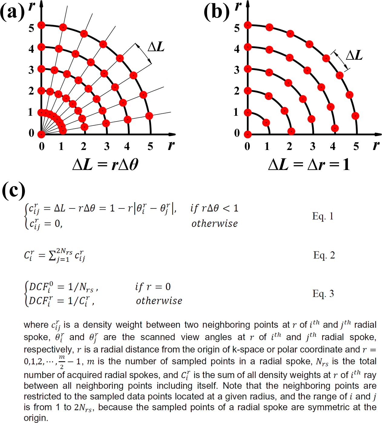
Optimized DCF: While each radial spoke samples uniformly-spaced discrete data points along the radial direction, the spacing along the circumferential direction between neighboring discrete points varies with the radius in the polar coordinate system (Figure-1a). We propose a new concept that the spacing along both the circumferential and radial directions is uniform such that $$$arc\;length\:(\triangle{L})=r\triangle{\theta}=\triangle{r}=1$$$ (Figure-1b), which is also a minimal spacing to avoid overlaps between samples at a given radius. Using this concept as a criterion, we propose to calculate the degree of overlap between two neighboring samples at a given radius. Specifically, a DCF at $$$r$$$ of $$$i^{th}$$$ radial spoke (i.e., $$$DCF_{i}^{r}$$$) can be calculated to be inversely proportional to the sum of density weights ($$$c_{ij}^{r}$$$) between all neighboring points including itself, as described in Figure-1c.
Phantom Experiment for FBP: We scanned a T1MES phantom³ on a 1.5T MRI system (Aera,Siemens), using a gradient echo pulse sequence with radial k-space sampling with the following imaging parameters: field-of-view (FOV)=288x288 mm², reconstruction matrix=192x192, slice thickness=8 mm, TE/TR=1.5/3.3 msec, receiver-bandwidth=1002 Hz/pixel, flip angle=15°, 600 radial spokes (i.e., full Nyquist condition), readout duration=2 sec, and dummy scan (2 sec). We separately acquired two data sets using regular-view angle=0.3° and tiny-golden-view angle=32.034°.⁴
In-vivo Experiment for CS: 48-fold accelerated, real-time PC data of 17 pediatric patients with CHD (10 males; mean age=11.3±3.2 years) were obtained from a previous study⁵ approved by our institutional review board. MRI scans included standard clinical 2D PC MRI with Cartesian k-space sampling (i.e., clinical PC) and real-time 2D PC MRI with radial k-space sampling (i.e., radial PC) at up to four locations (aortic valve, pulmonic valve, left-pulmonary artery, right-pulmonary artery; N=60 vascular planes in total). For the relevant imaging parameters of clinical PC, please see reference.⁵ The relevant imaging parameters for 48-fold accelerated, radial PC were: FOV=288x288 mm², reconstruction matrix=192x192, in-plane resolution=1.5x1.5 mm², slice thickness=6 mm, receiver-bandwidth=745 Hz/pixel, flip angle=12°, TE/TR=1.8/4.17 msec, prospective ECG-triggering, free-breathing scan time=3.34 sec (835-msec of dummy scan+2.50 sec) leading to 300 continuous radial spokes per plane, and golden-view angles=111.2461°.⁴ Velocity-encoding strength was matched to the clinical PC (150-400 cm/sec). For additional details, please see reference.⁵
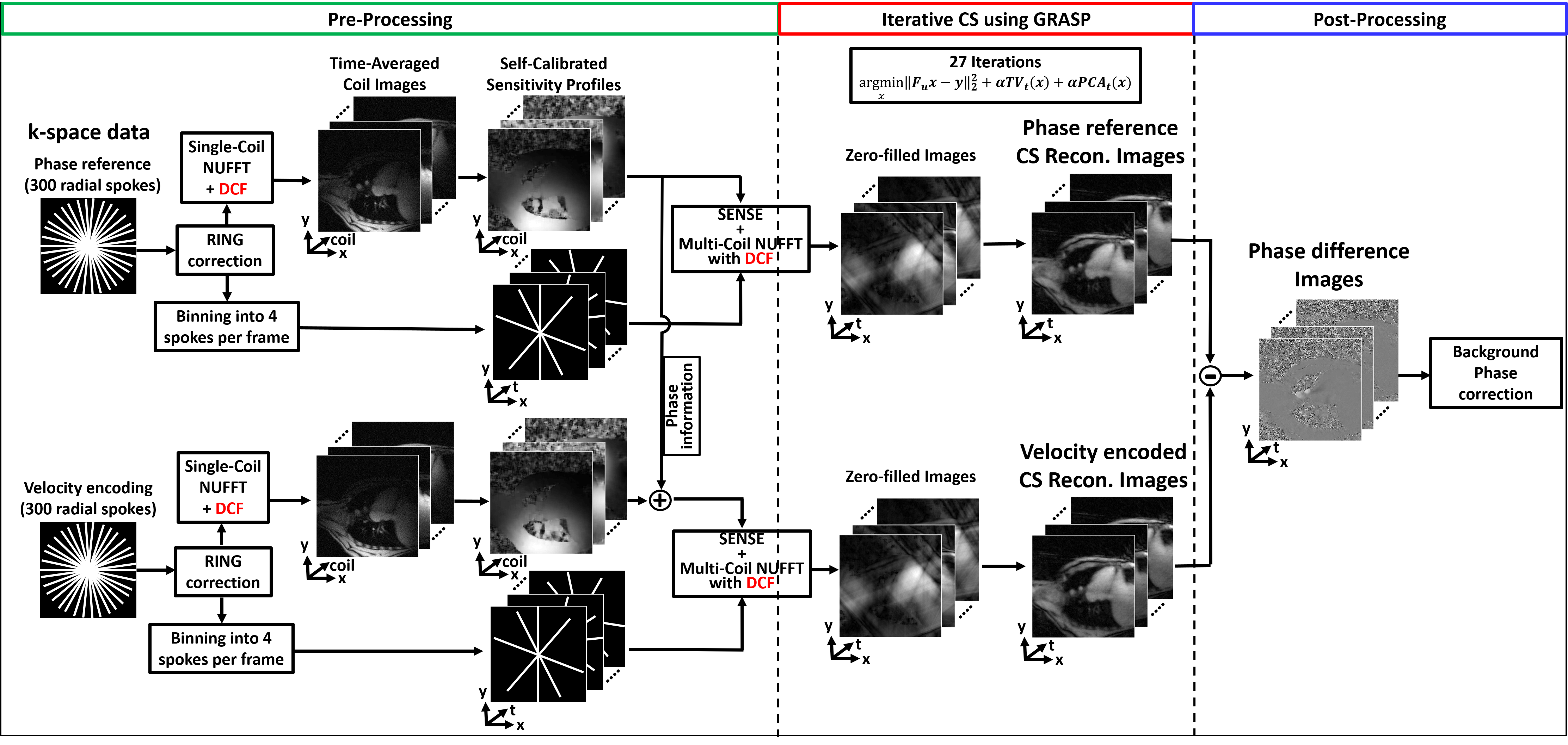
Image Reconstruction: All image reconstructions were separately performed using GPU-based non-uniform fast Fourier transform (NUFFT)⁶ with standard and optimized DCF on a GPU workstation (Tesla V100, NVIDIA) equipped with MATLAB (R2020b,MathWorks). Auto-calibrated gradient delay correction was performed on all k-space data using the RING method.⁷ For the phantom data reconstruction, FBP was performed using multi-coil NUFFT. For the patient data reconstruction, we binned 300 radial spokes to achieve 4 radial spokes per frame (33.4-msec temporal resolution) and employed a radial CS framework⁸ using two orthogonal sparsity transforms of temporal total variation (TV_t) and temporal principal component analysis (PCA_t) with identical normalized regularization weight (α)=0.0075 (relative to the maximum signal), as shown in Figure 2.
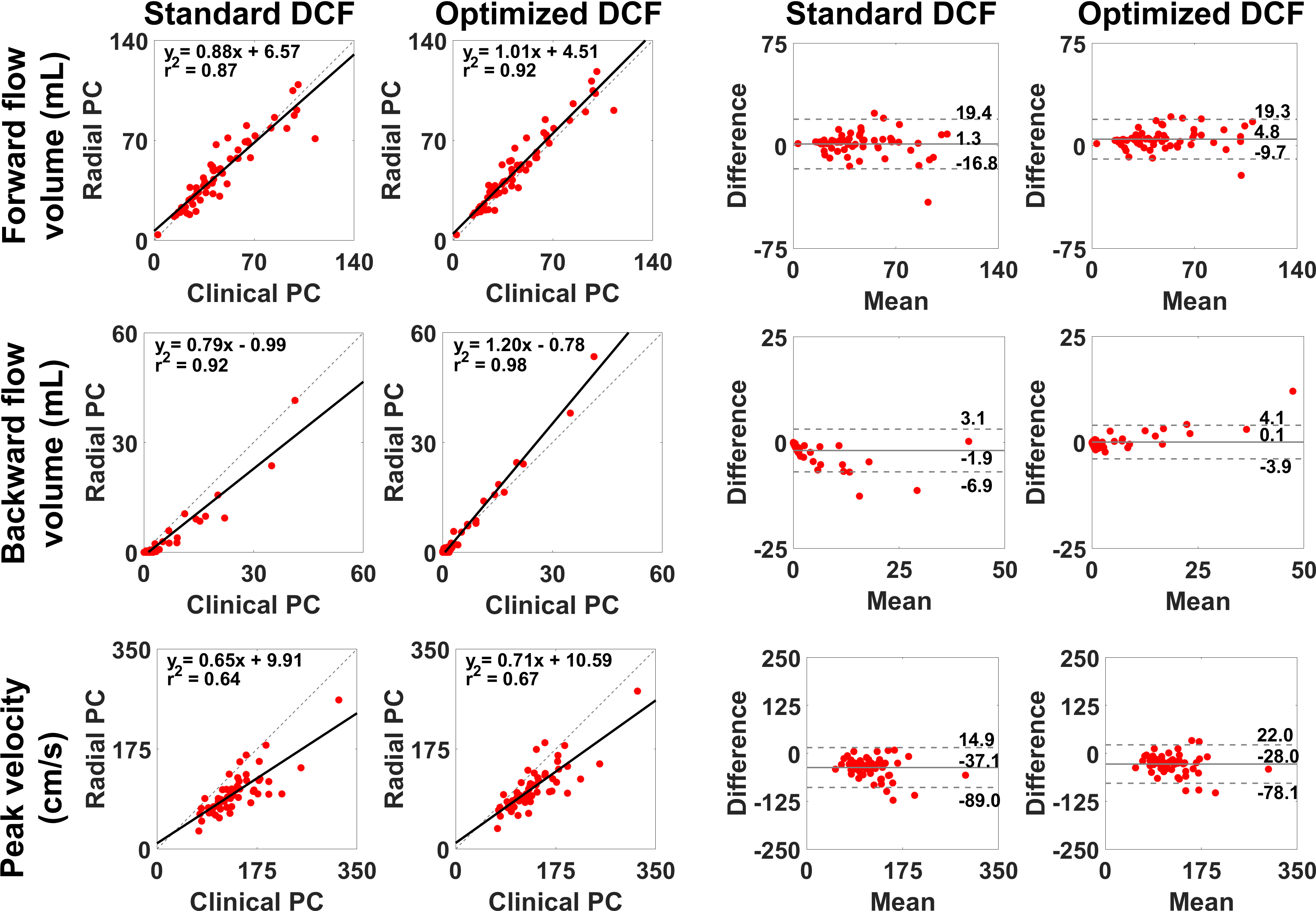
Image Analysis: For phantom data, we measured SNR. For in-vivo data, we quantified the forward-flow volume, backward-flow volume, and peak-velocity per location by manually drawing regions-of-interest in Matlab. For radial PC, we analyzed the first full-heartbeat in all subjects.
Statistical Analysis: We conducted linear-regression and Bland-Altman analyses on forward-flow volume, backward-flow volume, and peak-velocity to assess the degree of association and agreement, respectively, between clinical and radial PC datasets. p<0.05 was considered statistically significant.

Results

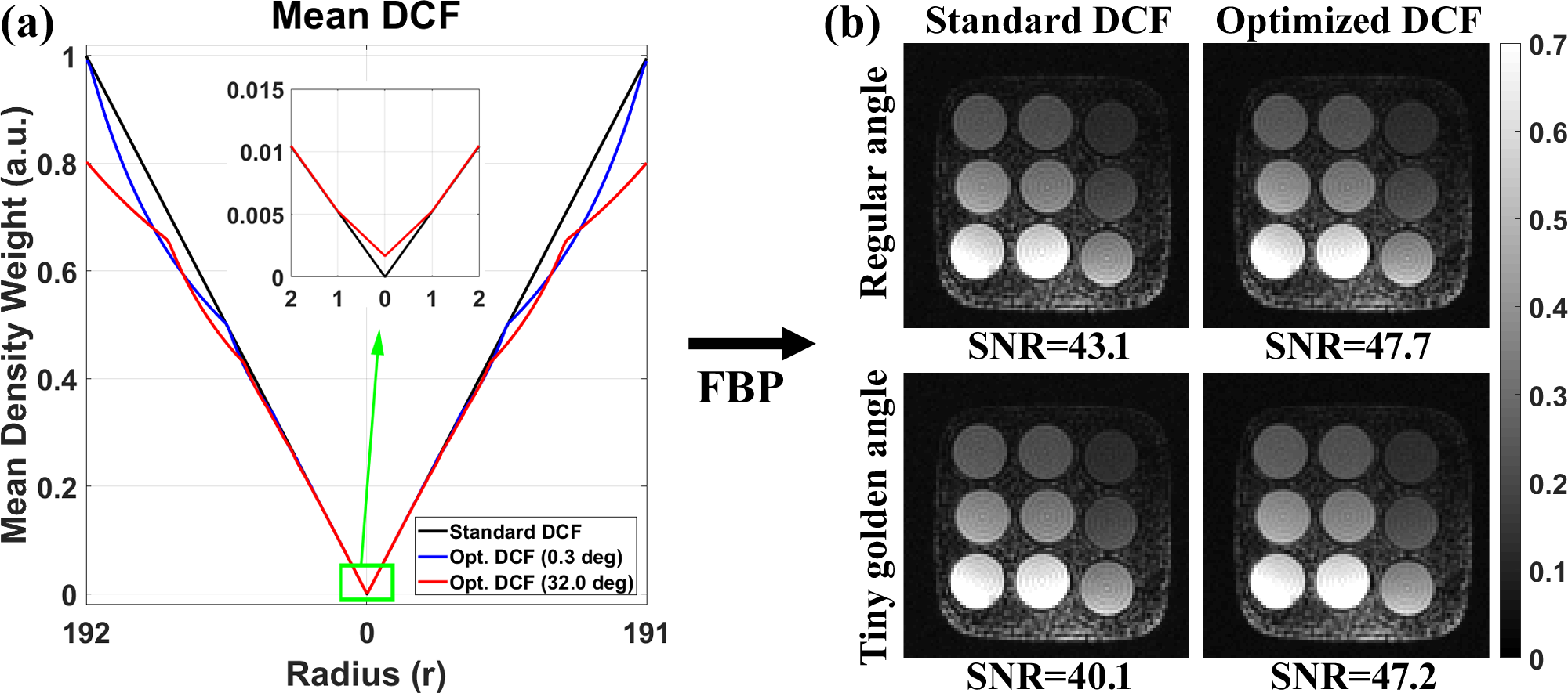
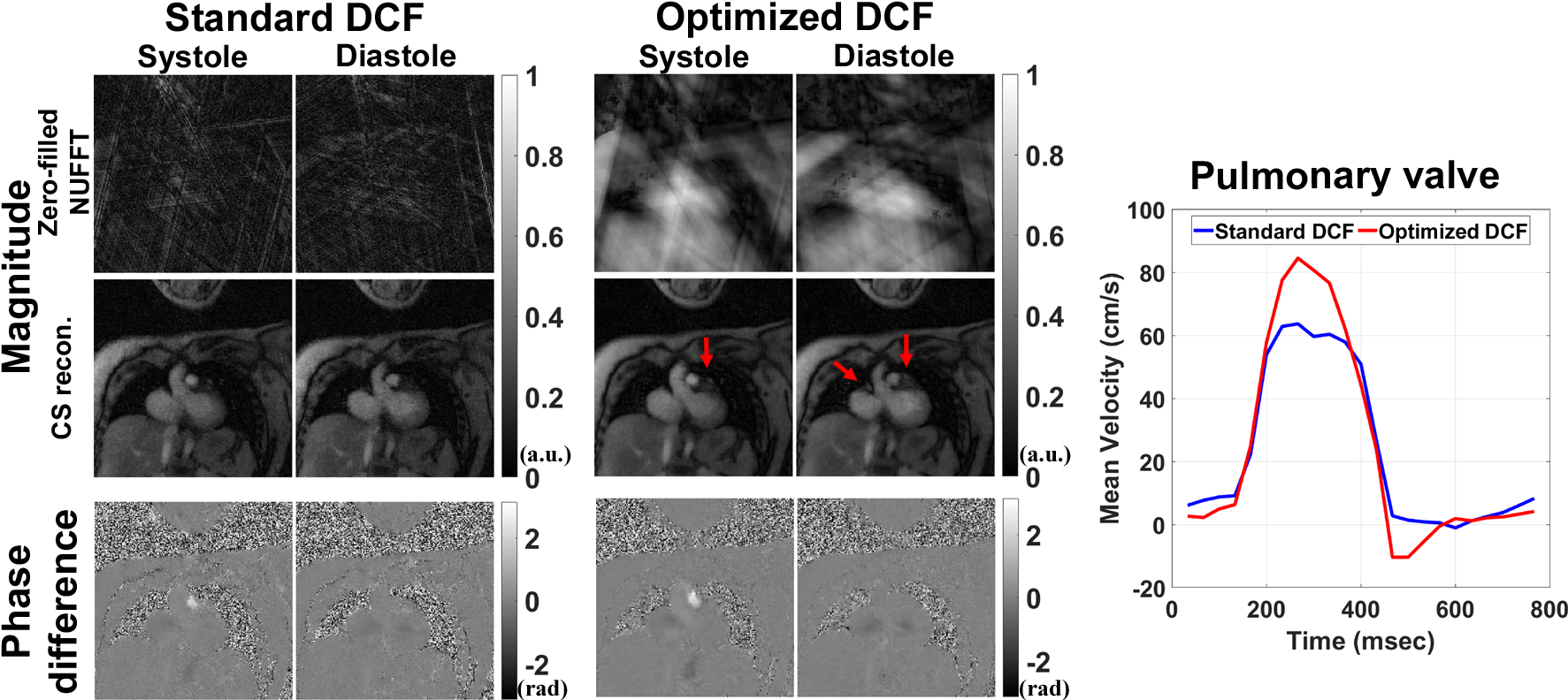
Figure 3a compares the mean DCF of 600 radial spokes between standard vs. optimized DCF. As shown in Figure 3b, the resulting FBP images of the phantom using optimized DCF produced 11 to 18% higher SNR than standard DCF for both regular and irrational-view angles. Figure 4 shows representative magnitude (zero-filled NUFFT and CS reconstruction) and phase-difference images in a pulmonary-valve plane, and the corresponding plots of mean velocity. Radial PC with optimized DCF produced higher dynamic range of mean velocity (i.e., less temporal blurring) than that with standard DCF. As shown in Figure 5, compared with clinical PC as reference, the levels of association and agreement in forward-flow volume, backward-flow volume, and peak-velocity were better for optimized DCF than standard DCF.

Discussions

This study demonstrates that optimized DCF produces higher SNR in FBP(phantom) and more accurate peak-velocity, forward-flow volume, and backward-flow volume in 48-fold accelerated radial PC MRI. Future work includes extending the optimized DCF for 3D radial scans.

Acknowledgements

This work was supported in part by the following grants: National Institutes of Health (R01HL116895, R01HL138578, R21EB024315, R21AG055954, R01HL151079) and American Heart Association (19IPLOI34760317).