2862

Correcting Signal Intensity Bias in ¹⁹F MR Imaging of Inflammation by Statistical Modelling

Ludger Starke¹, Thoralf Niendorf¹, and Sonia Waiczies¹
¹Berlin Ultrahigh Field Facility (B.U.F.F.), Max Delbrück Center for Molecular Medicine in the Helmholtz Association, Berlin, Germany

Synopsis

Labeling cells with ¹⁹F nanoparticles (NPs) continues to elicit interest for non-invasive localization of inflammation and monitoring immune cell therapy. Systematic overestimation in low SNR MRI of ¹⁹F-NPs has been previously described which needs to be corrected for valid quantitative conclusions. We develop a statistical model which successfully compensates this bias and demonstrate its efficacy for the correct estimation of signal intensities on neuroinflammation data acquired in a mouse model of multiple sclerosis. The correction only relies on the image data itself and promises to be a valuable contribution to the development of reliable quantitative ¹⁹F MRI.

Introduction

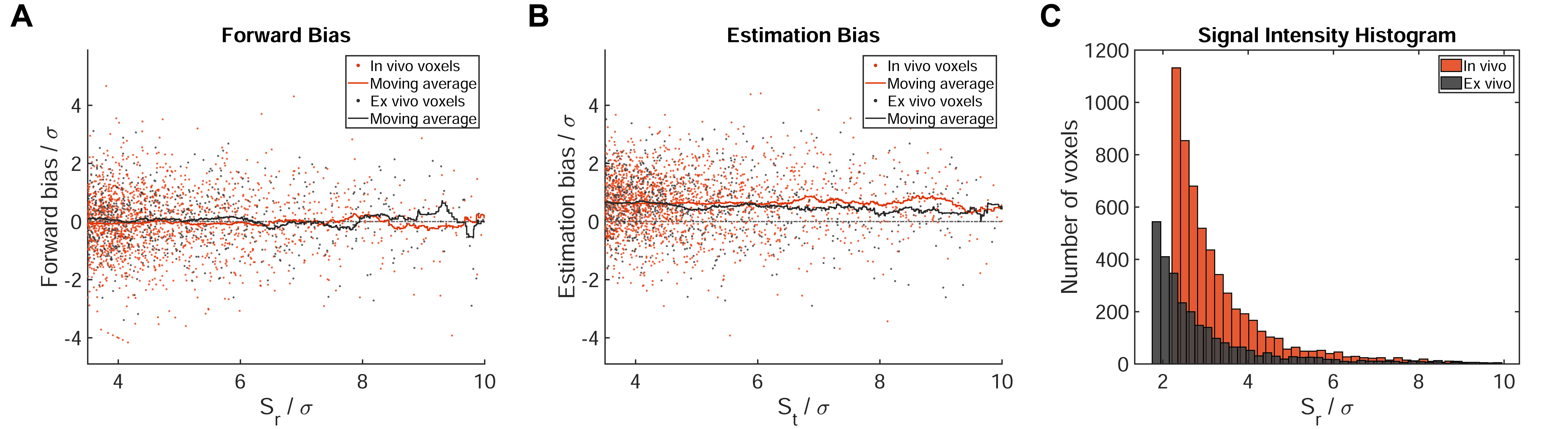
Labeling cells with ¹⁹F nanoparticles (NPs) continues to elicit interest for the non-invasive ¹⁹F MR localization of inflammation and monitoring immune cell therapy.^1,2 We recently reported strong bias in conventional, magnitude reconstruction ¹⁹F MRI when imaging inflammation in a mouse model of multiple sclerosis (experimental autoimmune encephalomyelitis, EAE).³ The effect occurred despite Rician noise bias correction (RNBC)⁴ and reduction of the observed bias will be essential for future quantitative applications of ¹⁹F MR. Statistical characteristics of the experiments were low SNR, no a priori known signal location, and a heavily skewed distribution of signal intensities (Fig.1). Here we propose a statistical model which successfully removes the bias without need for additional calibration experiments.

Methods

We examine 11 in vivo datasets from 5 SJL/J mice, partially scanned on multiple days, and ex vivo datasets from 5 different mice. Perfluoro-15-crown-5-ether rich nanoparticles were administered daily starting on day 5 following EAE induction⁵ and in vivo data was acquired on day 10 to 14. Ex vivo tissue was fixed and secured in tubes filled with paraformaldehyde.⁵
A 3D-RARE protocol was employed for ¹⁹F-MRI: TR=800ms, TE=4.4ms, ETL=40, FOV=(45x16x16)mm³, (140x40x40) matrix. 32min and 80min (in vivo) or 128min (ex vivo) measurements are used as test and reference data, respectively. Signal intensities after RNBC⁴ are denoted as S_t and S_r. The noise level σ was estimated based on a background region. Images were thresholded at SNR=3.5 and features of less than 3 connected ¹⁹F signal voxels were removed as outliers. For more details on the data, see also Starke et al., Setup 2 and 3.³
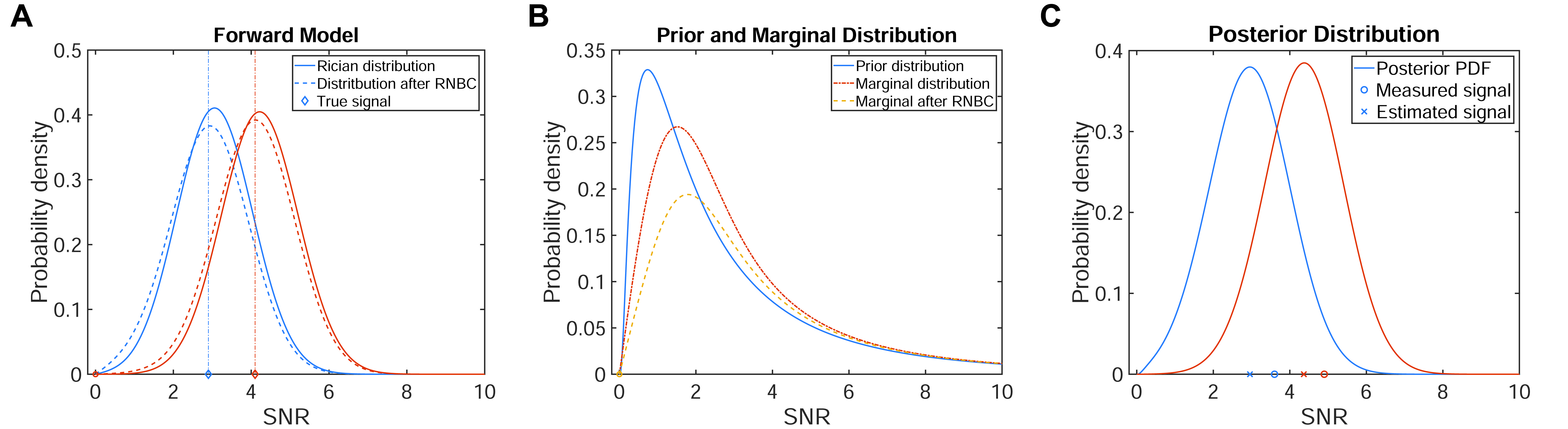
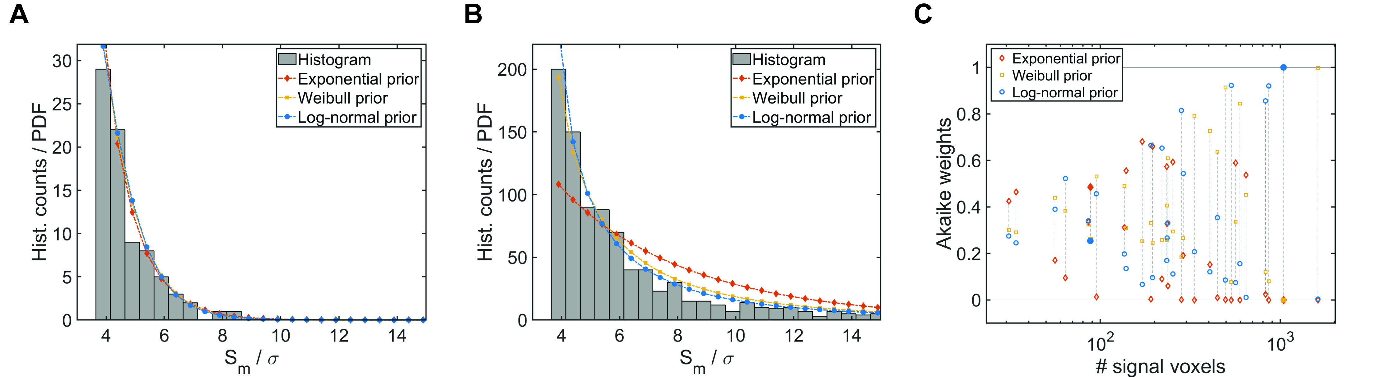
For true, but unknown signal S^* and measured signal S_m before RNBC , the forward model π_σ(S_t|S^*) is given by Rician distribution Ri(S_t;S_m,σ) (Fig.2a). We model S^* as drawn iid from prior distribution π_θ(S^*) with parameters θ and consider three different prior distributions commonly used for skewed data: exponential, Weibull and log-normal. We estimate θ for each image individually by maximizing the likelihood of the measured signal intensities under the marginal distribution π_σ,θ(S_m)=∫π_σ(S_m|S^*)π_θ(S^*)dS^* (Fig.2b). Akaike information criterion (AIC) weights were computed for all test and reference images to compare the prior distribution candidates.⁶ For all subsequent computations the log-normal prior was used.
Based on prior distribution and forward model, we computed the corrected signal as the posterior mean following Bayes theorem (Fig.2c). Analysis was performed by comparison of S_t and S_c to S_r for single voxels and averaged over complete features, i.e. separate clusters of connected signal voxels. To evaluate the effectiveness at different signal levels, a moving average with bin width 0.8σ was computed weighted by the number of voxels per feature.

Results

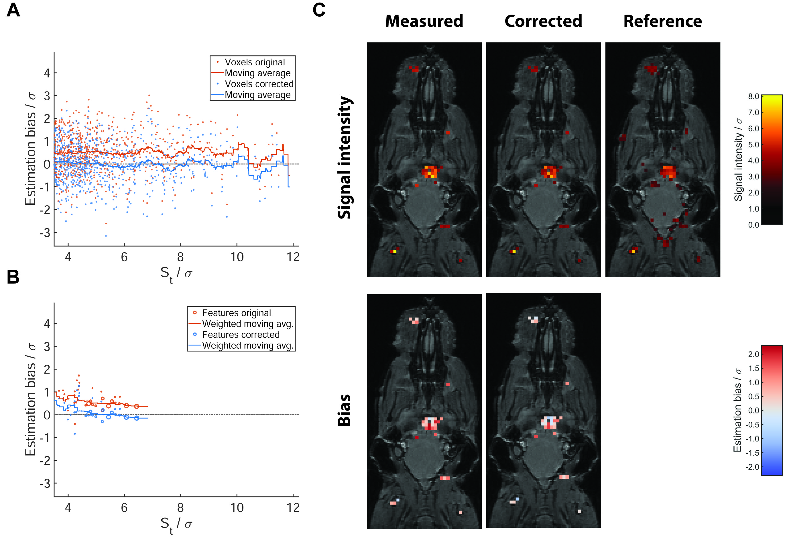
Marginals based on the Weibull and log-normal prior provided a good fit of the measured data for datasets with both small (Fig.3a) and large numbers of signal voxels (Fig.3b), whereas the exponential prior did not yield a good fit for multiple datasets spanning a larger range of signal intensities (Fig.3b). The Akaike weights show each of the candidates as optimal for some of the datasets. The single parameter exponential prior is favored in small datasets, whereas the Weibull and log-normal distribution are superior for larger datasets and perform similarly (Fig.3c).
In an example in vivo dataset, the signal intensity is overestimated at all signal levels by on average 0.5σ (Fig.4a). The model-based correction successfully removes this bias without altering the random spread (Fig.4a). The same holds true when averaging over signal features, except for those close to the detection threshold. No difference between smaller and larger features is noticeable (Fig.4b). The example slice (Fig.4c) illustrates these effects: while the change to the signal level of individual voxels is small, the corrected image contains a balance of overestimated and underestimated voxels, while the original nearly exclusively contains overestimated voxels.
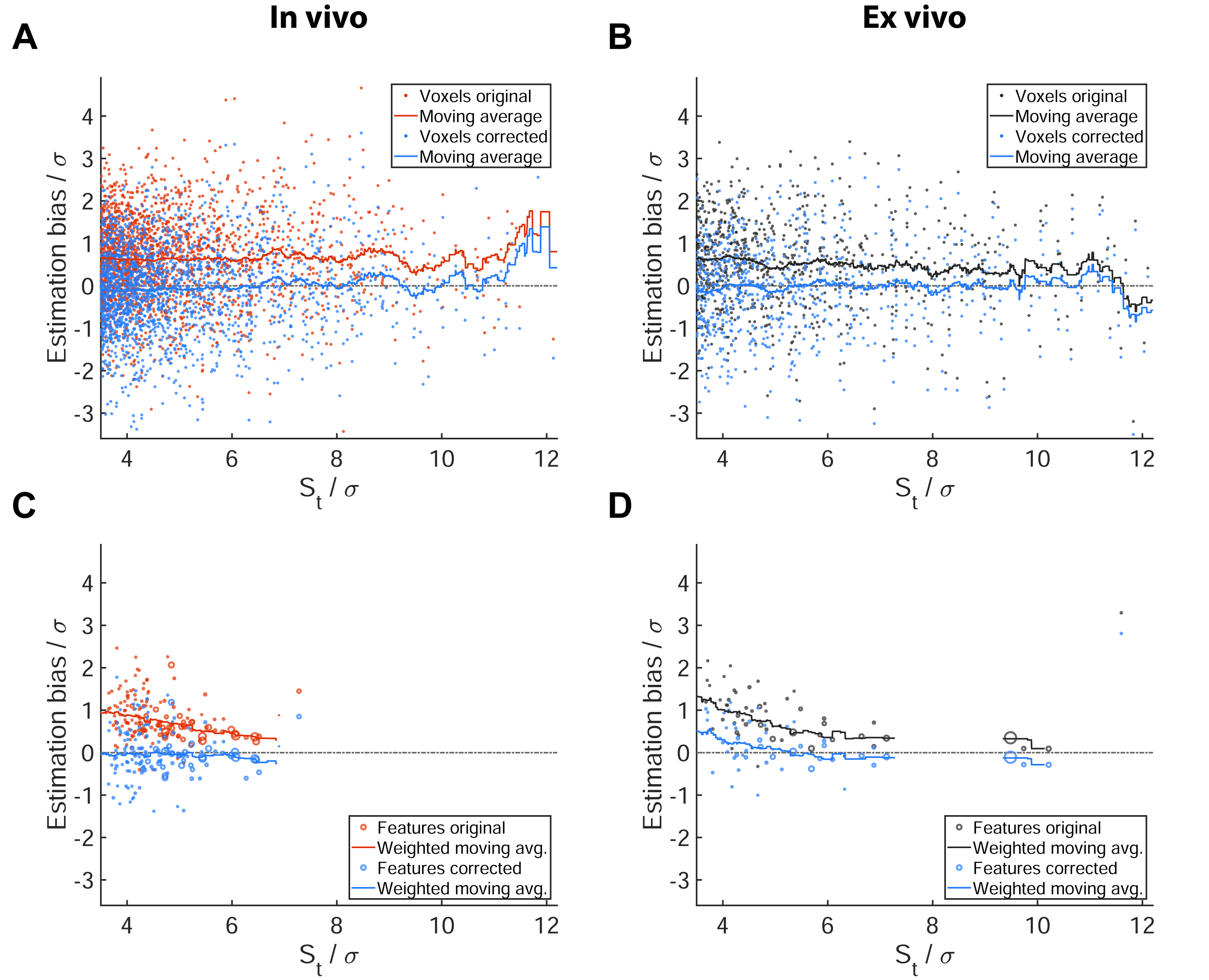
The joint analysis of all datasets confirms these observations (Fig.5). In vivo the average overestimation in uncorrected data is slightly larger than in the example at about 0.8σ (Fig.5a) for single voxels and up to 1σ averaged over features (Fig.5c). Again, the average bias in the corrected data is close to 0 except at S_t/σ>10, where few available voxels lead to fluctuations of the moving average. Analysis of the ex vivo data yields similar results (Fig.5b,d).

Discussion & Conclusion

We have shown that systematic overestimation in low SNR MRI of ¹⁹F-NPs can be explained and corrected by assuming that signal intensities are drawn from a heavily skewed distribution, e.g. a log-normal. While the effect size is below the random uncertainty for individual voxels, both the overestimation in uncorrected data and the effectiveness of model-based correction persist when averaging over ROIs, which would normally suggest a high degree of certainty. Thus, correction is essential to achieve quantitatively correct conclusions.
The correction can be applied purely in post-processing without the need to change data acquisition protocols. A natural extension of the existing model would be to exploit the spatial structure of imaging data, e.g. by modelling a hidden Markov random field. It remains to be investigated whether similar effects occur in other ¹⁹F MRI applications, such as the imaging and quantification of fluorinated drugs,⁷ or in different low SNR MR measurements.

Acknowledgements

This study was funded in part by the Deutsche Forschungsgemeinschaft to Sonia Waiczies (DFG WA2804). Thoralf Niendorf was supported by an advanced grant from the European Research Council (EU project 743077 - ThermalMR).

References

1. Darçot E, Colotti R, Pellegrin M, et al. Towards Quantification of Inflammation in Atherosclerotic Plaque in the Clinic - Characterization and Optimization of Fluorine-19 MRI in Mice at 3 T. Scientific reports. 2019;9(1):17488.

2. Chapelin F, Capitini CM, Ahrens ET. Fluorine-19 MRI for detection and quantification of immune cell therapy for cancer. J Immunother Cancer. 2018;6(1):105.

3. Starke L, Pohlmann A, Prinz C, Niendorf T, Waiczies S. Performance of compressed sensing for fluorine-19 magnetic resonance imaging at low signal-to-noise ratio conditions. Magn Reson Med. 2020;84(2):592-608.

4. Henkelman RM. Measurement of signal intensities in the presence of noise in MR images. Med Phys. 1985;12(2):232-233.

5. Waiczies S, Millward JM, Starke L, et al. Enhanced Fluorine-19 MRI Sensitivity using a Cryogenic Radiofrequency Probe: Technical Developments and Ex Vivo Demonstration in a Mouse Model of Neuroinflammation. Scientific reports. 2017;7(1):9808.

6. Wagenmakers EJ, Farrell S. AIC model selection using Akaike weights. Psychon Bull Rev. 2004;11(1):192-196.

7. Prinz C, Starke L, Millward JM, et al. In vivo detection of teriflunomide-derived fluorine signal during neuroinflammation using fluorine MR spectroscopy. In Press. Theranostics 2020. Doi:10.7150/thno.47130

Figures

(A) Distribution of signal levels after RNBC for given reference signal. Forward bias is defined as S_t(S_r) - S_r. Here no thresholding was applied to the test data. Conventional magnitude MRI on average leads to S_t(S_r) = S_t. (B) This does not guarantee unbiased estimation when trying to infer the true signal level from the measured signal. Estimation bias is defined as S_t - S_r(S_t). (C) The investigated animal model shows a distribution of signal intensities heavily skewed towards low signal intensity voxels. All 3 subfigures consist of data gathered from all investigated datasets.

(A) Rician noise with known noise level is used for the forward model. (B) The true signal intensities are assumed to be drawn from a positively skewed probability distribution. Here a log-normal prior is shown. The measured data is thus drawn from a marginal distribution computed by integrating the product of forward model and prior distribution. The right shift of probability mass for signal levels above the detection threshold leads to the observed overestimation. (C) Posterior distributions for two measured signal levels. The posterior mean gives the corrected signal

Comparison of prior distribution candidates. (A) In vivo test data. Signal intensity histogram and marginal distributions for 3 prior distribution candidates. Distribution parameters were estimated using maximum likelihood. (B) Analogous results for an ex vivo reference image. (C) Model selection. Akaike weights can be interpreted as the probability across the set of candidates that a model minimizes the information lost by adopting it. Filled markers represent the datasets shown in A and B.

Example in vivo dataset. Estimation bias including moving average for individual voxels (A) and averaged over signal features (B). The area of markers is proportional to the number of voxels in the feature. (C) Example slice from the same 3D dataset. ¹⁹F-NPs are taken up by inflammatory cells, which then accumulate at sites of inflammation. The first row shows ¹⁹F-MR signal intensity for test data after RNBC (measured) and with model based bias correction (corrected), as well as the reference data. The second line shows estimation bias computed by comparison of test and reference data.

Estimation bias analysis over all datasets. (A) In vivo single voxel, (B) ex vivo single voxel, (C) in vivo averaged over features, and (D) ex vivo averaged over features.

Proc. Intl. Soc. Mag. Reson. Med. 29 (2021)

2862