2838
Denoising Induced Iterative Reconstruction for Fast $$$T_{1\rho}$$$ Parameter Mapping1Research Center for Medical AI, SIAT, Chinese Academy of Sciences, Shenzhen, China, 2Paul C. Lauterbur Research Center for Biomedical Imaging, SIAT, Chinese Academy of Sciences, Shenzhen, China
Synopsis
We propose a novel DenOising induCed iTerative recOnstRuction framework (DOCTOR) to realize fast $$$T_{1\rho}$$$ parameter mapping from under-sampled k-space measurements. The proposed formulation constrains simultaneously intensity-based and orientation-based similarity between the reconstructed images and denoised prior images. Two state-of-art 3D denoising technologies are utilized including NLM3D and BM4D. The reconstruction alternates between two steps of denoising and a quadratic programming attacked by non-linear conjugate gradient method. The parameter maps are created from the reconstructed images using conventional fitting with an established relaxometry model. Through experiments in-vivo $$$T_{1\rho}$$$-weighted brain MRI datasets, we can observe superior image-quality of the proposed DOCTOR scheme.
Introduction
The observation forward model for accelerated scanning can eventually be approximated as a discretized linear system:$$Y=\mathcal{A}X+N$$where $$$X\in \mathbb{C}^{U\times W}$$$ denotes the desired image series to be reconstructed. $$$W$$$ is the total number of spin-lock time (TSL). The observed k-space data is given as $$$Y\in \mathbb{C}^{V\times W}$$$. The linear operator $$$\mathcal{A}:\mathbb{C}^{U\times W}\rightarrow\mathbb{C}^{V\times W}$$$ formulates the observation forward model which performs a multiplication by coil sensitivities followed by an undersampled Fourier transform in each column. The backward program of reconstructing $$$X$$$ is an ill-posed problem by the reason that the problem is underdetermined with $$$V \ll U$$$ . By adding penalty function to a cost function, the variational formulation for this inverse problem can be written as: $$\min_{X}\frac{1}{2}\parallel\mathcal{A}X-Y\parallel^{2}_{2}+\lambda\mathcal{H}(X)$$where the penalty function $$$\mathcal{H}(X)$$$ enforces some a priori knowledge about the image series $$$X$$$, which usually acts as a regularization depended on transform-coefficient sparsity$$$^{1,2}$$$, low-rank nature$$$^{3,4}$$$or the combinations$$$^{5,6}$$$.Method
In the paper, we propose a novel DenOisinginduCed iTerative recOnstRuction framework (DOCTOR) to accelerate $$$T_{1\rho}$$$ parameter mapping from under-sampled k-space measurements. The parameter maps will be created subsequently from the reconstructed images using conventional fitting with an established relaxometry model. We specify the main iteration of our reconstruction algorithm as follows:$$\boldsymbol{Step~1}:X^{\mathcal{D}}=\mathcal{D}enoising(X,\sigma);\\~~~~~~~~~~~~~~~~~~~~~~~~~~~~~~~~~~~~~~~~~~~~~~~~~~~~~~~~~~~~~~~~~~~~~~~~~~~~~~~\boldsymbol{Step~2}:\min_{X}\frac{1}{2}\parallel\mathcal{A}X-Y\parallel^{2}_{2}+\lambda\sum_{i}^{fov}(\parallel X_{i}-X^{\mathcal{D}}_{(i)}\parallel_{2}^{2}+\alpha\parallel (\mathcal{G}X)_{i}\times(\mathcal{G}X^{\mathcal{D}})_{(i)}\parallel_{2}^{2})$$where $$$\boldsymbol{Step~1}$$$ denotes a denoising step for 3D MR images with multiple TSLs. The step aims to progressively induce $$$X^{\mathcal{D}}$$$ as prior-image series, which have underlying image structures enforced by the powerful denoising model. $$$\sigma$$$ is the strength-parameter of denoising, which is varied to gradually uncover image structures. In $$$\boldsymbol{Step~2}$$$, a quadric optimization with observation fidelity can be directly attacked using non-linear conjugate gradient (NLCG) algorithm. The two $$$l_{2}$$$-norm based regularizing terms enforce the intensity-based and orientation-based similarity between the reconstructed image and denoised prior images in each iterative process. $$$\lambda$$$ is the trade-off parameter. $$$\alpha$$$ is used to control the contribution of orientation-based similarity prior. $$$\mathcal{G}$$$ represents the 3D gradient operator. A multi-scale gradients $$$^{7}$$$ in the horizontal and vertical directions are given as: $$\mathcal{G}_{h}x=\frac{1}{J}\sum_{j=1}^{J}\frac{x(s+j,t)-x(s,t)}{\sqrt{j}};\\\mathcal{G}_{v}x=\frac{1}{J}\sum_{j=1}^{J}\frac{x(s,t+j)-x(s,t)}{\sqrt{j}}$$where $$$J$$$ is the scale number. $$$s$$$ and $$$t$$$ are the row and column index. When $$$J$$$ is large, the response of gradient on edges is large and the tiny difference of weak edges in denoised prior images can be effectively captured. Moreover, the symbol $$$\times$$$ represents the cross product, and the cross product of vectors $$$u$$$ and $$$ v$$$ is defined as a determinant: $$u\times v=\begin{vmatrix} \boldsymbol{i} & \boldsymbol{j} & \boldsymbol{k}\\ u_{1} & u_{2} & u_{3}\\ v_{1} & v_{2} & v_{3}\end{vmatrix}=(u_{2}v_{3}-u_{3}v_{2})\boldsymbol{i}-(u_{1}v_{3}-u_{3}v_{1})\boldsymbol{j}+(u_{1}v_{2}-u_{2}v_{1})\boldsymbol{k}$$The determinant has magnitude zero when the vectors are parallel.Experiment
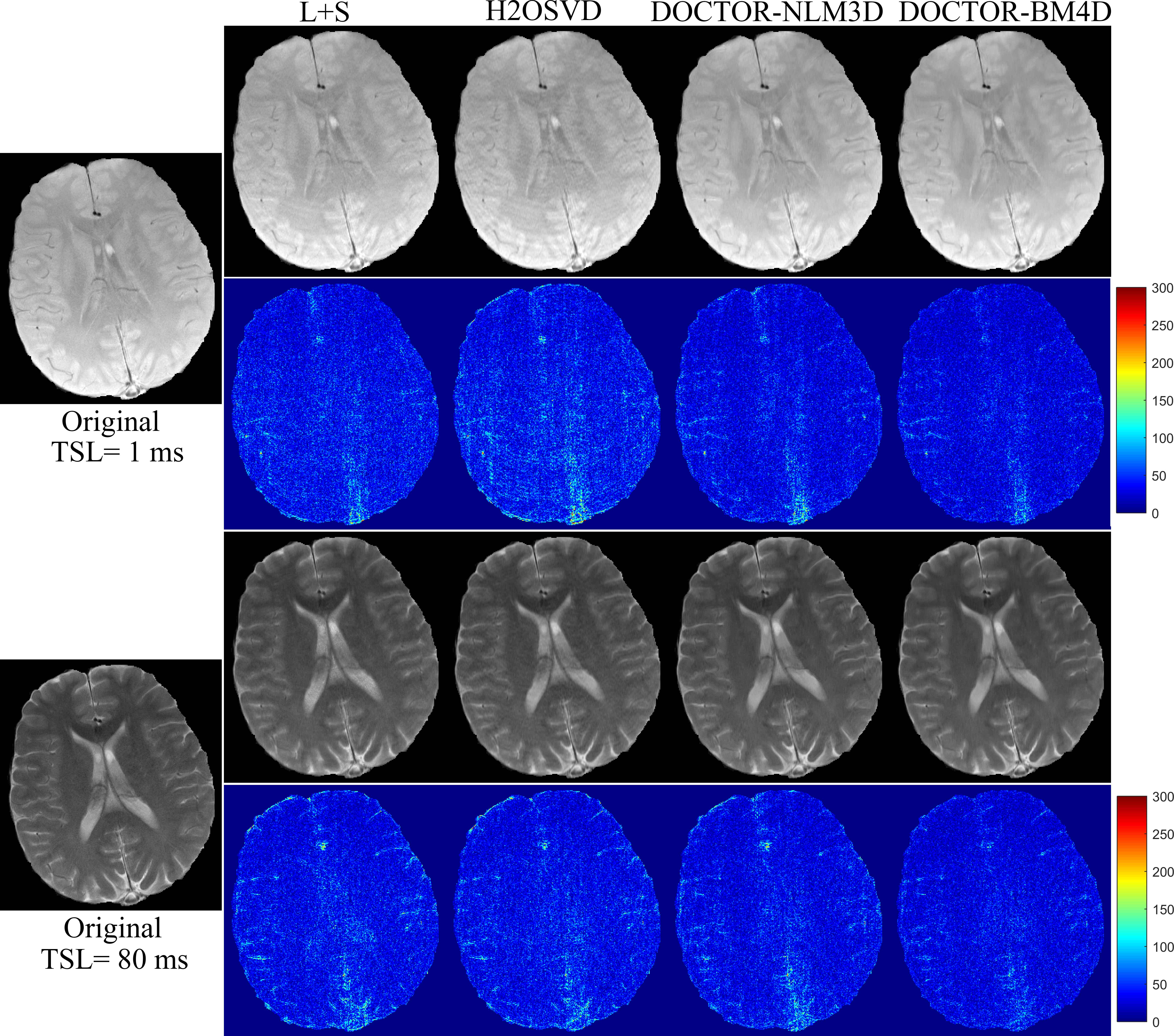
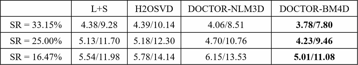
The experiments are carried out on $$$T_{1\rho}$$$-weighted brain MR images (TE = 7ms, TR = 3000ms, excitation pulse flip angle =90°, refocusing pulse flip angle =180°, echo train length =16, pixel size =0.6 × 0.6 mm2, matrix size =768368, slice thickness =5mm, and TSLs =1, 20, 40, 60, and 80ms). 1D variable density random under-sampling pattern is adopted to generate sampled k-space data. We compare our reconstructions using the L+S $$$^{8}$$$ and Hankel-HOSVD (H2OSVD). Two state-of-art 3D MR image denoising technologies based on block matching and filtering are adopted including NLM3D $$$^{9}$$$ and BM4D $$$^{10}$$$. All reconstructions were performed in Matlab R2017a on a standard laptop (Windows 10, 64 bit operation system, Intel(R) Core(TM) i7-9700 CPU, 3 GHz, 32 GB RAMS). The reconstruction quality is quantified with the relative error (RE), which are defined as RE$$$=\frac{\parallel X-\hat{X}\parallel_{2}}{\parallel X\parallel_{2}}\times 100\%$$$, where $$$X$$$ and $$$\hat{X}$$$ denote the fully-sampled original image series and the reconstructed image series, respectively.Results
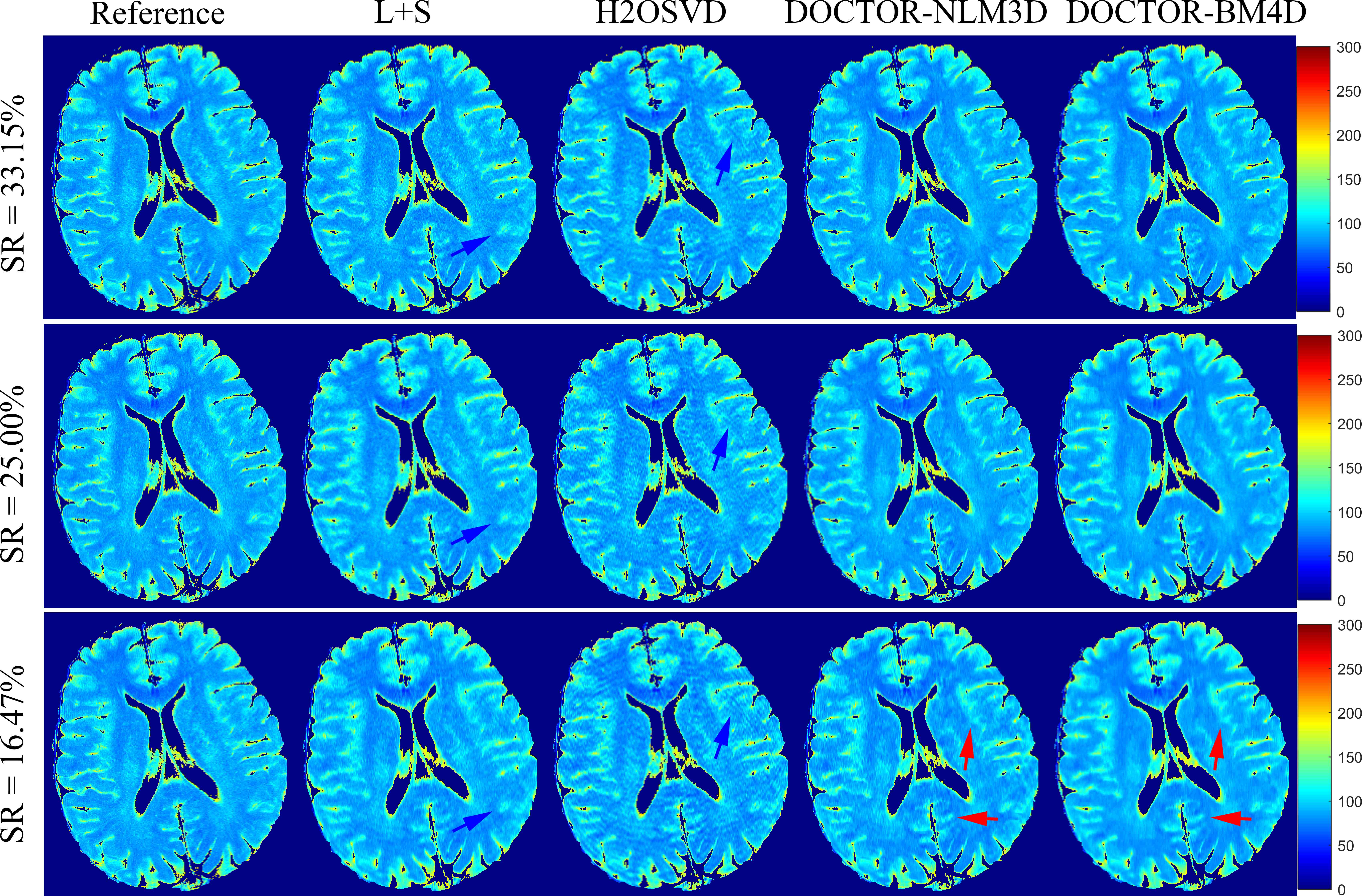
Figure 1 shows the reconstruction results of all comparison methods at TSL=1ms and TSL= 80ms with sampling ratio (SR) of 25.00$$$\%$$$. Among them, the returned images of the H2OSVD method has unacceptable artifacts (indicated by the blue arrow), and the L+S method has a relative good result than H2OSVD. However, L+S still produces some visible blurs. As expected, the DOCTOR based reconstructions have superior performances: the DOCTOR-NLM3D and DOCTOR-BM4D methods both further sharpen the images and suppress the artifacts. It is not difficult to see from the error maps that the DOCTOR-BM4D method can define more fine details (indicated by the red arrow). Figure 2 shows that the DOCTOR methods achieve the parameter maps with higher quality compared with the L+S and H2OSVD methods at SR=16.47$$$\%$$$, 25.00$$$\%$$$ and 33.15$$$\%$$$. The RE values of the reconstruction images and parameter maps using all methods at different SRs are listed in the Figure.3. The DOCTOR methods, especially DOCTOR-BM4D, have lower RE values than other methods.Conclusion
In the paper, we propose a DOCTOR framework to accelerate $$$T_{1\rho}$$$ parameter mapping. Experimental results prove the effectiveness and superiority of the proposed DOCTOR methods.Acknowledgements
This work was supported in part by the National Key R&D Program of China (2017YFC0108802 and 2017YFC0112903); National Natural Science Foundation of China (61771463, 81830056, U1805261, 81971611, 61871373, 81729003, 81901736); Natural Science Foundation of Guangdong Province (2018A0303130132); Key Laboratory for Magnetic Resonance and Multimodality Imaging of Guangdong Province; Shenzhen Peacock Plan Team Program (KQTD20180413181834876); Innovation and Technology Commission of the government of Hong Kong SAR (MRP/001/18X); Strategic Priority Research Program of Chinese Academy of Sciences (XDB25000000).References
- Doneve M, Brnert P, Eggers H, et al. Compressed sensing reconstruction for magnetic resonance parameter mapping. Magnetic Resonance in Medicine. 2010; 64(4): 1114-1120.
- Velikina J V, Alexander A L, Samsonov A. Accelerating MR parameter mapping using sparsity-promoting regularization in parametric dimension. Magnetic Resonance in Medicine. 2013; 70(5): 1263-1273.
- Zhang T, Pauly J M, Levesque I R. Accelerating parameter mapping with a locally low rank constraint. Magnetic Resonance in Medicine. 2015; 73 (2): 655-661.
- Park S H, Jin K, Hwan K, et al. Acceleration of MR parameter mapping using annihilating filter based low rank hankel matrix (ALOHA). Magnetic Resonance in Medicine. 2016; 76(6): 1848-1864.
- Zhao B, Lu W, Hitchens T K, et al. Accelerated MR parameter mapping with low-rank and sparsity constraints. Magnetic Resonance in Medicine. 2015; 74 (2): 489-498.
- Zhu Y J, Liu Y, Ying Leslie Y, et al. SCOPE: signal compensation for low-rank plus sparse matrix decomposition for fast parameter mapping. Physics in Medicine & Biology. 2018; 63(18):185009(16pp).
- Zhu Q, Wang W, Cheng J, et al. Incorporating reference guided priors into calibrationless parallel imaging reconstruction. Magnetic Resonance Imaging. 2019; 57:347-358.
- Otazo R, Emmanuel C, and Daniel K S. Low-rank plus sparse matrix decomposition for accelerated dynamic MRI with separation of background and dynamic components. Magnetic Resonance in Medicine. 2015; 73(3): 1125-1136.
- Manjon J V, Coupe P, Bonmati L M, et al. Adaptive non-local means denoising of MR images with spatially varying noise levels. Journal of Magnetic Resonance Imaging. 2010; 31(1): 192-203.
- Maggioni M, Katkovnik V, Egiazarian K, et al. Nonlocal transform-domain filter for volumetric data denoising and reconstruction. IEEE Transaction on Image Processing. 2013; 22(1): 119-133.
Figures