Introduction

Arterial Spin Labeling (ASL) is a promising imaging technique for the quantitative analysis of brain function and development. However, one of the greatest challenges affecting the reliability of ASL measurement is its relatively low Signal-to-Noise Ratio (SNR). A long scan time is needed to acquire a perfusion image with sufficient SNR. Reducing the number of measurements results in a decrease in SNR. Deep Learning (DL) methods have been applied to ASL image denoising in several previous studies, and most studies focused on denoising using the spatial features only^2,3. However, temporal feature is also an important characteristic for ASL as it contains a time series of perfusion measurements. Long-short-term Memory (LSTM) is a network structure designed to learn features of the sequential data, which has the potential to perform denoising based on temporal features. In this study, we developed a novel DL algorithm to perform spatial-temporal ASL denoising with convolutional neural network (CNN) combined with convolutional LSTM (ConvLSTM) to improve SNR of ASL images with fewer input time steps.

Methods

1. Data acquisition and preprocessing
We studied 162 pCASL datasets acquired in 121 children between the age of 7 to 18 years (62M) from the Pediatric Template of Brain Perfusion database⁵. Images were acquired on a Siemens 3T Trio scanner using 2D EPI sequence (TR/TE=4000/12 ms, resolution 3.125×3.125×6 mm³, labeling duration 1.5s and post labeling delay 1.2s). A total of 40 control and label pairs were acquired. Data preprocessing included the following steps. First, all of the raw images were corrected for rigid head motion, perfusion image series were generated by pairwise subtraction between label and control acquisitions and were then normalized to the standard MNI space. The second step was image intensity standardization, which linearly mapped the image intensity values according to a population histogram¹. The purpose of this step was to remove the bias between datasets and make the model easier to learn noise features. The ground truth perfusion images were generated by averaging across all the 40 perfusion image series. 80% of the whole dataset was randomly chosen to be used as the training set, 10% as the validation set and the rest as the test set.

2. Network and training
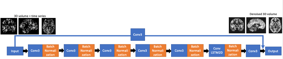
We implemented a CNN and ConvLSTM based network using the keras platform (keras.io). Figure 1 shows the network structure of the model. The network consisted of a global pathway and a local pathway with five layers of 3D convolutional layers and one layer of convolutional LSTM. The convolutional layers were used to capture the 3D spatial features of the image and the ConvLSTM layers were used to capture the spatiotemporal features of the perfusion image series. Each individual time step of input image was served as a channel to the input layer, and at the output, a single denoised image was produced and used to calculate the loss. Mean square error was used as the loss function and rectified linear unit (ReLU) was used as the activation function. Different time steps (20, 15, 10, 5) were used as the input to test the robustness of the model. Each of these models used the same structure and learning rate except the number of input channels. The training of each model took about 8 hours.

3. Model evaluation
The trained models were used to predict the denoised image from the test data sampled with the same input time steps. We evaluated results by calculating the Peak-Signal-to-Noise Ratio (PSNR) and Structural Similarity Index (SSIM) of the predicted denoised image and the “ground truth” 40-time-steps-averaged image on the test set. The mean PSNR and mean SSIM values were calculated across the test datasets. The results were also compared with the average of input image series fed to the models and the result using PCA-based denoising algorithm⁴.

Results and Discussion

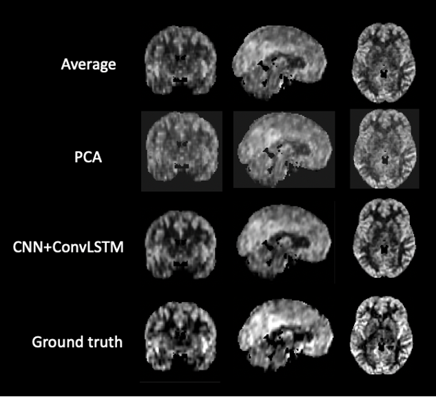
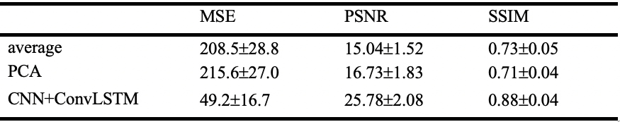
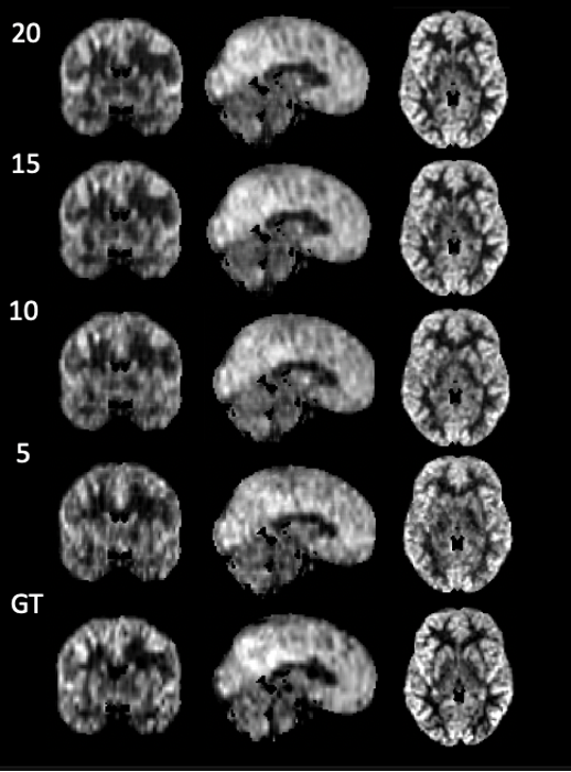
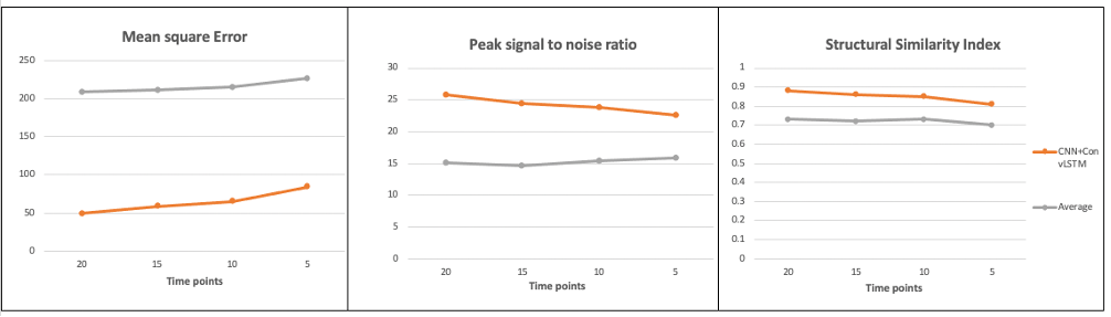
Figure 2 shows the result of one individual dataset with 20-time-steps input (half of the full-time series). The output image of the CNN +ConvLSTM model showed excellent quality along all of the three axes compared to the ground-truth. Table 1 shows the statistical results of the model output compared to averaging and denoising with PCA. The results show that our DL algorithm can provide better results compared to traditional methods with the highest PSNR and SSIM (p-value < 0.0001). Figure 3 shows the output images of the model when fed separately with different numbers of input time steps as compared to the ground-truth on a representative subject. Figure 4 plots the performance metrics of the models fed with different input time steps, in which the proposed model outperformed the average method at all the time steps. With a fewer number of input time steps, the performance of denoising declined slightly in a linear fashion, which indicates that the use of more information may improve the model prediction.

Conclusion

Our model combining CNN with Convolutional LSTM for spatiotemporal ASL denoising can achieve an SNR improvement with fewer input time steps, which shows a potential to reduce the scan time for ASL acquisition. Further studies are needed to see if the proposed DL denoising algorithm can provide better quantitative analysis for brain perfusion.

Acknowledgements

No acknowledgement found.