2722
Clinically applicable automatic quantitative renal perfusion measurement using ASL-MRI and machine learning1Center for Image Sciences, University Medical Center Utrecht, Utrecht, Netherlands, 2Department of Radiology, University Medical Center Utrecht, Utrecht, Netherlands
Synopsis
ASL-MRI quantification involves kidney segmentation and cortex-medulla differentiation to obtain cortical renal blood flow, requiring time consuming manual interaction hampering clinical adoption. We applied machine learning to automat renal ASL-MRI quantification. A cascade of three U-nets was constructed to replace manual segmentation steps. Automatic segmentation yielded a dice score of 0.78, which was similar to the inter-observer variability of 0.77. Moreover, good agreement for cortical RBF was found between automatic and manual segmentations on group and individual level; 211±31 and 208±31mL/min/100g, respectively. Our proposed method automates quantification without compromising performance. This makes renal ASL-MRI more attractive for clinical application.
INTRODUCTION
Clinical applicability of renal ASL-MRI is hampered due to time consuming and observer dependent post-processing. In order to obtain accurate cortical renal blood flow (RBF), renal cortex segmentation is needed, requiring time consuming manual interaction.1,2 State-of-the-art methods in renal ASL literature, are often intensity-based thresholding approaches requiring manual intervention.3–7 However, machine learning has proven its value in medical image segmentation in several organs,8 including the kidneys.9,10 This study aims to investigate the accuracy of automatic renal cortex perfusion quantification by including deep learning-based segmentation.METHODS
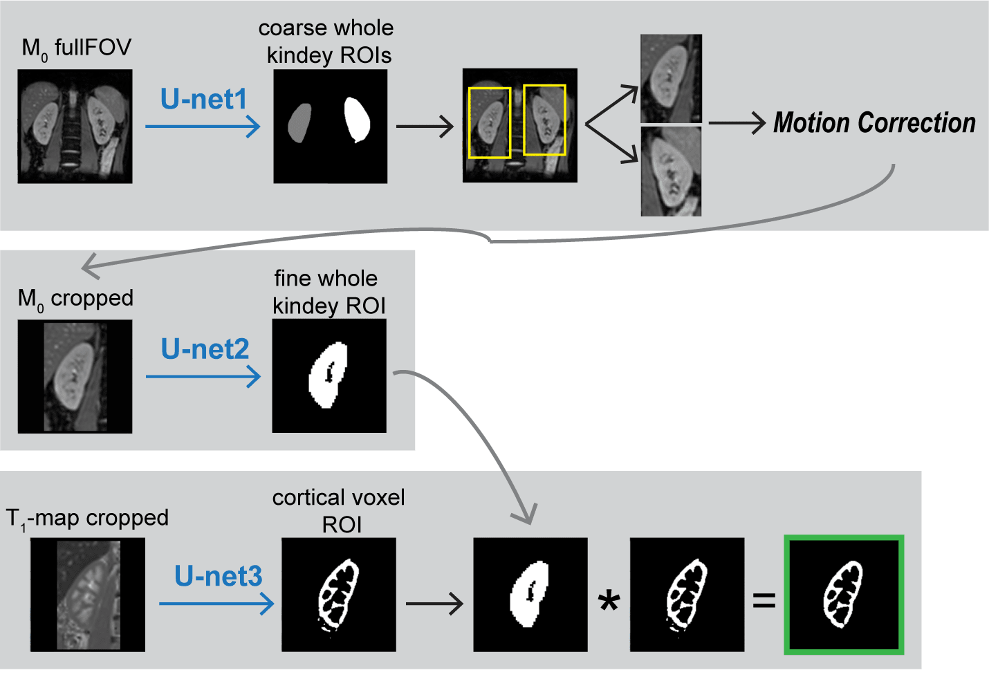
Data: ASL-MRI data were acquired on a 1.5T MRI scanner (Ingenia, Philips, The Netherlands) using single-shot multi-slice gradient echo EPI with a spatial resolution of 2.56 x 2.56 x 6mm and five coronal slices covering the kidney. Each ASL dataset per volunteer consisted of an M0-image, a T1-map and ASL-images (pseudo continuous ASL with background suppression). For training and cross validation data from 10 healthy volunteers was used (Dataset1). For validation of the trained cascade performance on an independent test set, data of 4 additional volunteers was used (Dataset2).Manual segmentations were obtained through pixelwise labeling by two observers, yielding a reference and a second observer set. Per subject, manual segmentation of both kidneys took about 20 minutes. Prior to training, all images were resampled to an in-plane-resolution of 1x1mm, followed by zero padding to a squared FOV.Cascade: The cascade is illustrated in Figure 1.
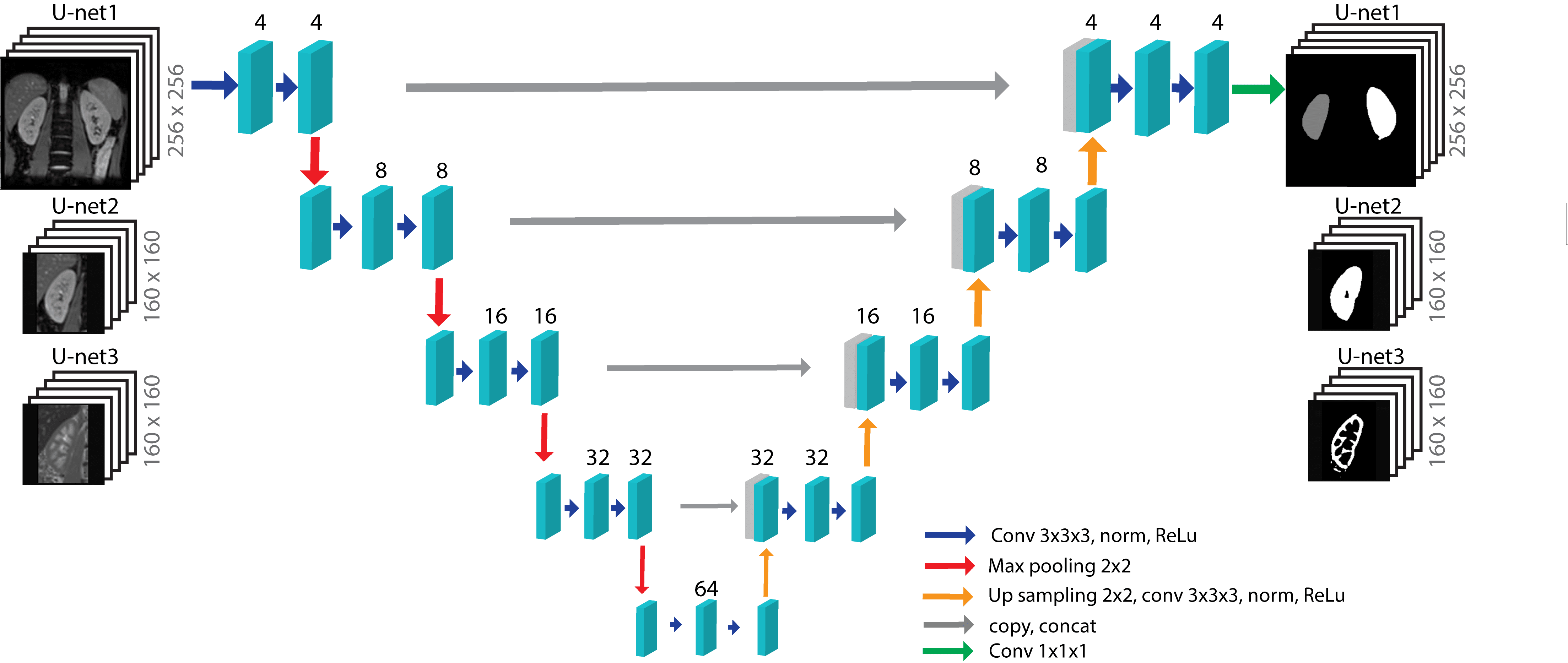
Architecture: Figure 2 shows the architecture of all U-nets.
Evaluation: Cascade performance evaluation was based on cortical dice score (DS, %), Hausdorff distance (HD, mm) and volumetric difference (VD, auto – manual, %). To validate the accuracy of using automatic cortical ROI definition for renal ASL quantification, cortical RBF mL/100g/min was quantified per subject using the automatic and manual cortical ROIs. RBF was quantified by ASL signal modelling using Buxton’s continuous model.11 Differences were tested using paired t-tests (α=0.05) and Bland-Altman analysis.
RESULTS
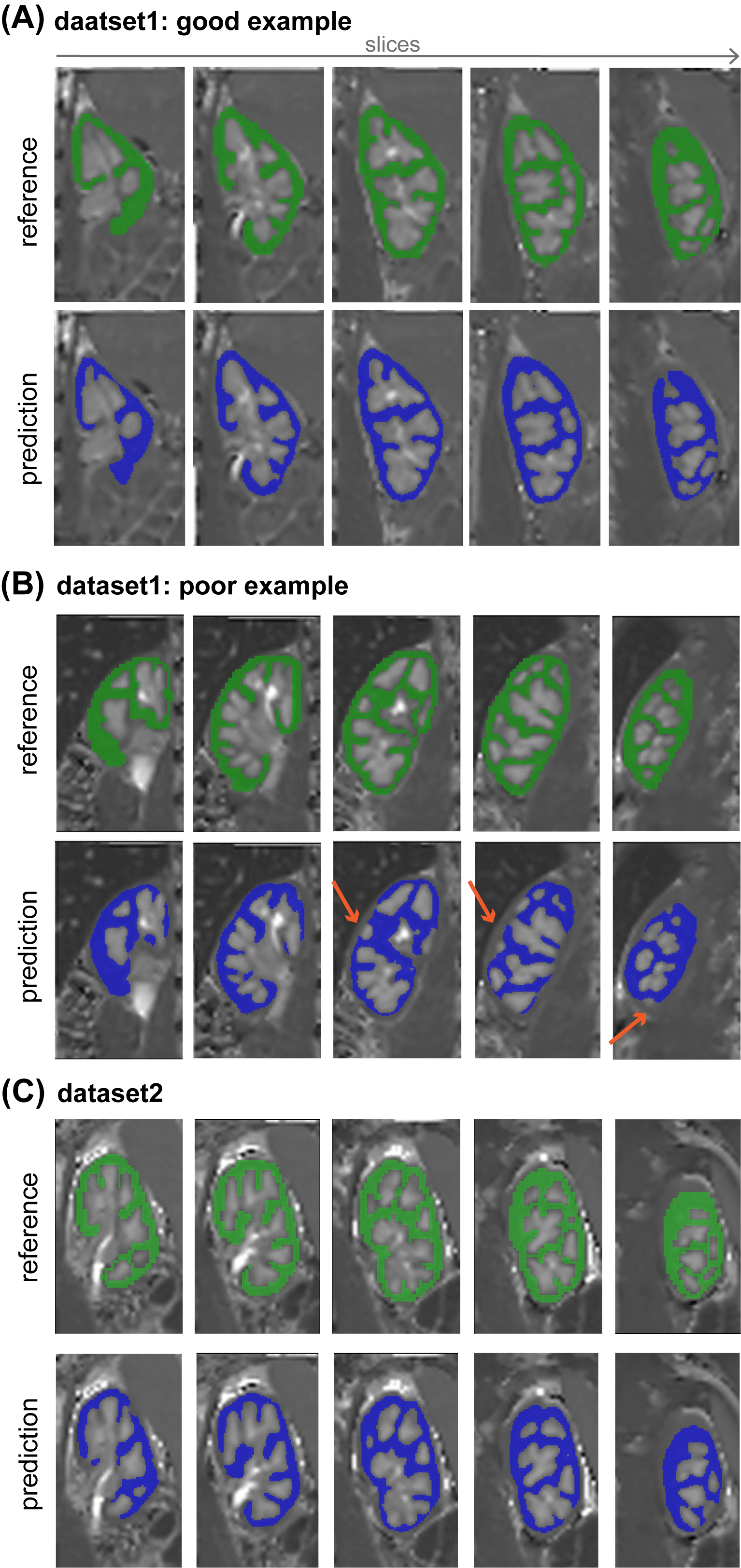
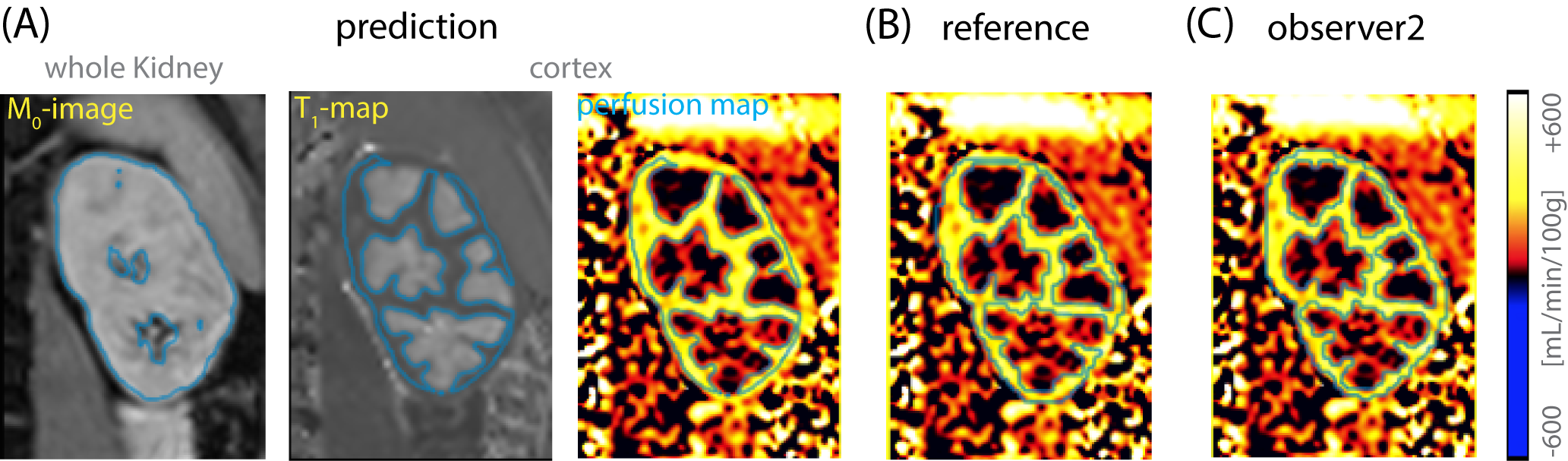
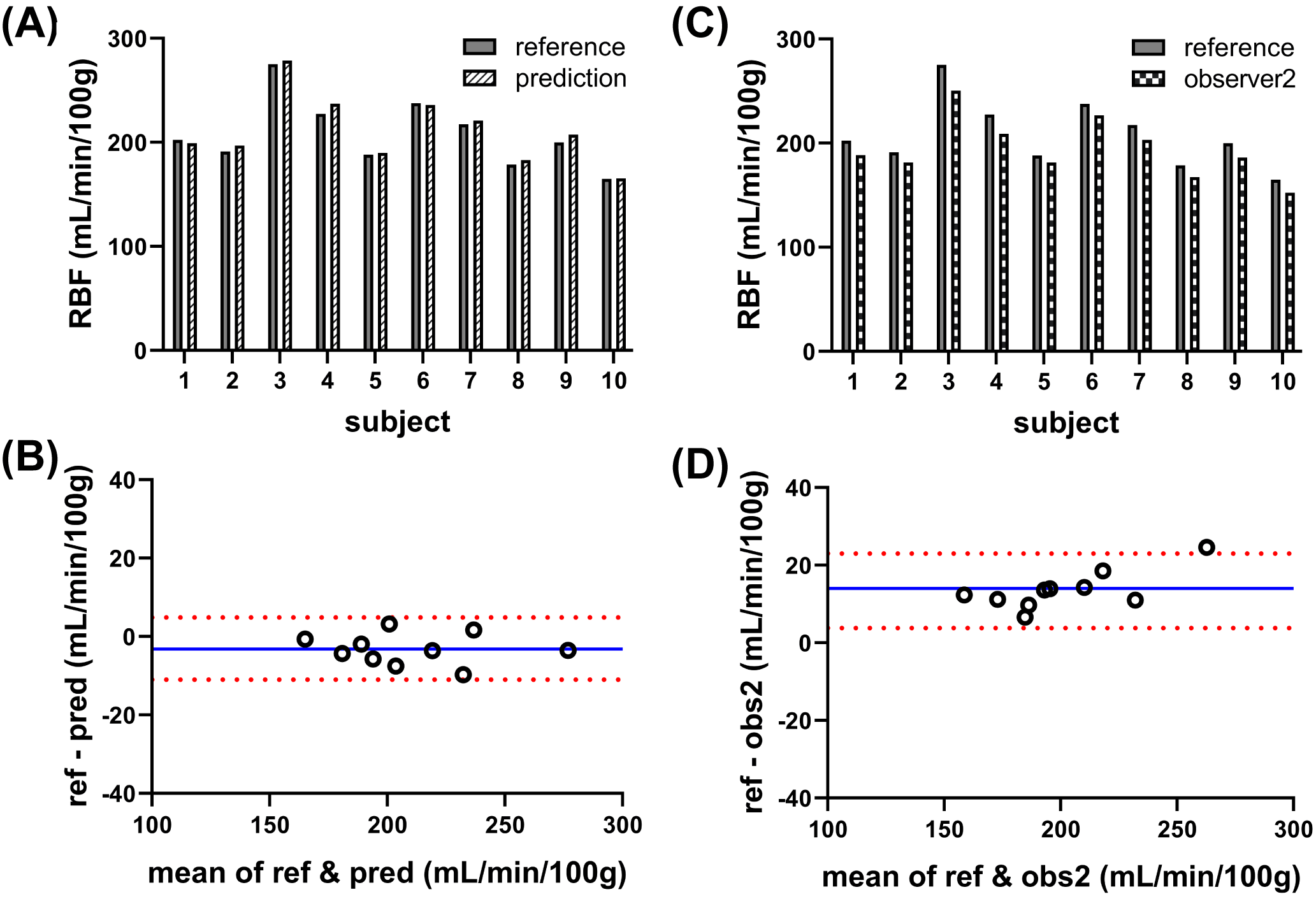
Qualitatively, good agreement was found between automatic and manual segmentation in cross-validation experiments (illustrated in Figure 3A-B). The cross-validation on Dataset1 yielded an average DS of 0.78±0.04, HD=6.3±5.4mm and VD=-9.6±5.4%. Between the two manual observers, cortical segmentations yielded comparable DS of 0.77±0.02 and HD of 8.5±4mm and a slightly larger volumes by observer 2: VD of 27.7±5.6%. Testing the trained cascade on an independent Datatset2 yielded results which are in line with training and cross-validation as well as inter-observer variability stated above (Figure 3C); DS of 0.75±0.03, HD of 7±1.7mm and VD of 20±5.6%.An example of the use of the segmentations for extraction of the cortical ASL quantification pipeline is illustrated in Figure 4. The fully automatic pipeline yielded cortical RBF values which were in line with using the manual reference, on average as well as on individual level (Figure 5A&B), with 211±31mL/min/100g and 208±31mL/min/100g (p<0.05), respectively, accompanied by narrow limits of agreement at -11 and 4.6mL/min/100g resulting from Bland-Altman analysis (Figure 5B). Interobserver variability was higher, on average and also on individual level (Figure 9D); with a lower average RBF of 195±27mL/min/100g (p<0.05) and limits of agreement of 3.8 and 23ml/min/100g (Figure 9D). The RBF accuracy with automated segmentations was confirmed on the independent Dataset2, resulting in an accurate cortical RBF, which was slightly but significantly higher than based on manual segmentations: 262±33ml/min/100g vs 248±32mL/min/100g, respectively (p<0.05).
DISCUSSION & CONLUSION
We demonstrate the feasibility of automatic renal cortex segmentation using machine learning for fully automatic ASL quantification. Predictions showed good agreement with the manual reference (dice = 0.78), which was in line with inter-observer variability (dice=0.77). Regarding ASL quantification, similar cortical RBF values were obtained when using automatic or manual segmentations, even on individual patient level. Likewise, good agreement was found when the trained cascade was tested on an independent dataset (dice=0.75).Generally, reported dice scores in this study are lower than comparable reports in literature, such as Couteaux et al. 201910 with a dice score of 0.87 on CT images. It should be noted that the high non-convexity of the cortical shape and the low resolution of the M0-images and T1-maps result in relatively many partial volume voxels, challenging the manual and automated segmentation and consequently decrease dice scores.
Differences in quantified cortical RFB using automatic or manual masks were small, but significant, which underlines consistency of the method among volunteers.
The proposed segmentation cascade approach for automatic renal ASL quantification should be applicable on ASL datasets acquired using a different readout sequence or with a different scanner. It is not to be excluded that additional preprocessing steps or training of the U-nets may be required.
Fully automatic processing of renal ASL-MRI could improve robustness of especially longitudinal and multi-center renal ASL studies as observer dependence is removed. Additionally, the proposed automatic method operates much quicker than manual observers and importantly removes the dependence on manual input in the processing. Consequently, renal ASL-MRI could be better applicable in clinical practice. Though, a larger subject group, including patients, is needed to evaluate the actual clinical performance of our proposed automatic method.
Acknowledgements
This work is part of the research program Applied and Engineering Sciences with project number 14951 which is (partly) financed by the Netherlands Organization for Scientific Research (NWO). We thank MeVis Medical Solutions AG (Bremen, Germany) for providing MeVisLab medical image processing and visualization environment, which was used for image analysis.References
- Nery F, Buchanan CE, Harteveld AA, et al. Consensus-based technical recommendations for clinical translation of renal ASL MRI. Magn Reson Mater Physics, Biol Med. 2020;33(1):141-161.
- Wu WC, Su MY, Chang CC, Tseng WYI, Liu KL. Renal perfusion 3-T MR imaging: A comparative study of arterial spin labeling and dynamic contrast-enhanced techniques. Radiology. 2011;261(3):845-853.
- Buchanan C, Cox E, Francis S. Evaluation of 2D Imaging Schemes for Pulsed Arterial Spin Labeling of the Human Kidney Cortex. Diagnostics. 2018;8(3):43.
- Bones IK, Franklin SL, Harteveld AA, et al. Influence of labeling parameters and respiratory motion on velocity-selective arterial spin labeling for renal perfusion imaging. Magn Reson Med. 2020;84(4):1919-1932.5.
- Cox EF, Buchanan CE, Bradley CR, et al. Multiparametric renal magnetic resonance imaging: Validation, interventions, and alterations in chronic kidney disease. Front Physiol. 2017;8(SEP):1-15. doi:10.3389/fphys.2017.006966.
- Gardener AG, Francis ST. Multislice perfusion of the kidneys using parallel imaging: Image acquisition and analysis strategies. Magn Reson Med. 2010;63:1627-1636.7.
- Harteveld AA, de Boer A, Franklin SL, Leiner T, van Stralen M, Bos C. Comparison of multi-delay FAIR and pCASL labeling approaches for renal perfusion quantification at 3T MRI. Magn Reson Mater Physics, Biol Med. 2020;33(1):81-94.8.
- Hesamian MH, Jia W, He X, Kennedy P. Deep Learning Techniques for Medical Image Segmentation: Achievements and Challenges. J Digit Imaging. 2019;32(4):582-596.
- Isensee F, Jäger PF, Kohl SAA, Petersen J, Maier-Hein KH. Automated Design of Deep Learning Methods for Biomedical Image Segmentation. 2019:1-55.
- Couteaux V, Si-Mohamed S, Renard-Penna R, et al. Kidney cortex segmentation in 2D CT with U-Nets ensemble aggregation. Diagn Interv Imaging. 2019;100(4):211-217.
- Buxton RB, Frank LR, Wong EC, Siewert B, Warach S, Edelman RR. A General Kinetic Model for Quantitative Perfusion Imaging with Arterial Spin Labeling. Magn Reson Med. 1998;40:383-396
Figures