2688
1D Convolutional Neural Network for Estimating BOLD Signal from Oscillating Steady State Signal1Biomedical Engineering, University of Michigan, Ann Arbor, MI, United States, 2Electrical Engineering and Computer Science, University of Michigan, Ann Arbor, MI, United States
Synopsis
Oscillating steady state imaging (OSSI) for fMRI commonly combines images across a fast oscillation to produce a steady time series suitable for fMRI analysis. The signal magnitude derived from L2-norm combination can be sensitive to frequency variations, which can exacerbate physiological noise, particularly respiration. Here, we use a 1D convolutional neural network (1DCNN) to directly estimate the underlying T2* BOLD response from both simulated and real OSSI fMRI signals. We demonstrated that our technique reduces B0 fluctuations and thermal noise as compared to the L2-norm combined OSSI fMRI signal.
Introduction
Unlike bSSFP 1 which uses balanced gradients with constant RF phase increments, OSSI uses balanced gradients with quadratic RF phase increments to generate a high SNR $$$T_2^*$$$-weighted signal that oscillates with a periodicity of $$$n_c\times TR$$$, where $$$n_c$$$ is the number of RF phase cycles used ($$$\sim$$$6-10) 2. The presence of oscillations in the OSSI signal produces banding artifacts that reduce the attainable SNR of a given image. These oscillations can be averaged out to produce a more uniform signal by combining the $$$n_c$$$ RF phase cycled images, using combination metrics such as the $$$L_2$$$-norm combination. The signal magnitude derived from the $$$L_2$$$-norm combination of the OSSI signal is sensitive to respiratory induced frequency fluctuations, which increase with decreasing $$$n_c$$$ values. The frequency sensitivity of the combined image can amplify physiological noise, leading to a deterioration in the overall signal quality. In order to circumvent the frequency sensitivity issues associated with OSSI signal combination, we designed a 1D convolutional neural network (1DCNN) to extract the underlying $$$T_2^*$$$ BOLD fMRI time course from 1D OSSI signals without explicitly combining the signal.Methods
We trained our 1DCNN(Fig.2&3) using data from Bloch simulations of the OSSI signal. Monte Carlo sampling was performed to randomly sample OSSI simulation parameters to diversify the neural network training data. Fig.1A shows the parameters that were sampled and their respective ranges. Twenty six unique 30s long blocked designs were simulated, where the blocked designs were convolved with a canonical hemodynamic response function (HRF) from SPM 3 to form the 45s BOLD responses. The BOLD responses were converted to $$$T_2^*$$$-weighted BOLD time courses by scaling the signal based on activation and baseline $$$T_2^*$$$ values.The OSSI signal was simulated for 626 isochromats with frequencies ranging between $$$-TR/2:0.1:TR/2$$$Hz. The scan parameters used are shown in Fig.1B. Different complex OSSI signals were created using different $$$T_2$$$ values, respiration B0 shifts, and respiration rates. To compute the $$$T_2^*$$$-weighted OSSI signal, the complex OSSI signal was weighted using a Cauchy distribution centered at a particular off-resonance frequency, with the peak width determined by the $$$T_2^′$$$ value. $$$T_2^′$$$ values are drawn from the BOLD curve, where a high $$$T_2^′$$$ value would produce a narrow Cauchy distribution, while a low $$$T_2^′$$$ value would produce a wide Cauchy distribution. The weighted OSSI signal was summed across all isochromats and complex additive Gaussian noise of $$$0.25\%$$$ of the maximum signal was added to the signal.
Lastly, the absolute value of the complex weighted signal was computed and used for training/testing the neural network. In total, 4200 different BOLD signals and their corresponding $$$T_2^*$$$-weighted OSSI fMRI signals were generated. Fig.1 shows a flow chart that summarizes the data sampling and OSSI simulation pipeline. The combined signals from taking the $$$L_2$$$-norm of the OSSI signals across $$$n_c$$$ cycles were also computed to compare to the neural network results.
OSSI signals from human subjects were acquired using a single-slice, single-shot constant density spiral out trajectory ($$$n_c= 6$$$, $$$TR=17.5$$$ms, flip angle $$$=10^\circ$$$, FOV $$$= 19 \times 19 cm^2$$$, matrix $$$=45 \times 45$$$, slice thickness = 2.5mm and sampling BW = 250kHz). The functional task was a right- and left-hemifield counter-phased 10Hz flickering checkerboards in 40s blocks, repeated 6 times (240s). More information about real data and fMRI experiments can be found in Cao et al 4
Results
[Simulations]Fig.4A-D compares BOLD signals from the 1DCNN combined, $$$L_2$$$-Norm combined, and the ground-truth $$$T_2^*$$$ values from our simulation data. These figures show that our 1DCNN significantly reduces signal distortions from respiration, off-resonance frequency, and thermal noise as compared to the BOLD signal from $$$L_2$$$-norm combination. Moreover, the correlation coefficient between the 1DCNN BOLD signal and the ground truth BOLD signal is greater than 0.6 in more than 90% of the simulated data compared to the $$$L_2$$$-norm combined signal, where approximately 23% of the data had correlation coefficient greater than 0.6. In Fig.4E, the NRMSE for 1DCNN BOLD signal was 0.6% which is substantially lower compared to the NRMSE of 2.6% from the $$$L_2$$$-norm combined BOLD signal.
[Human Subject]
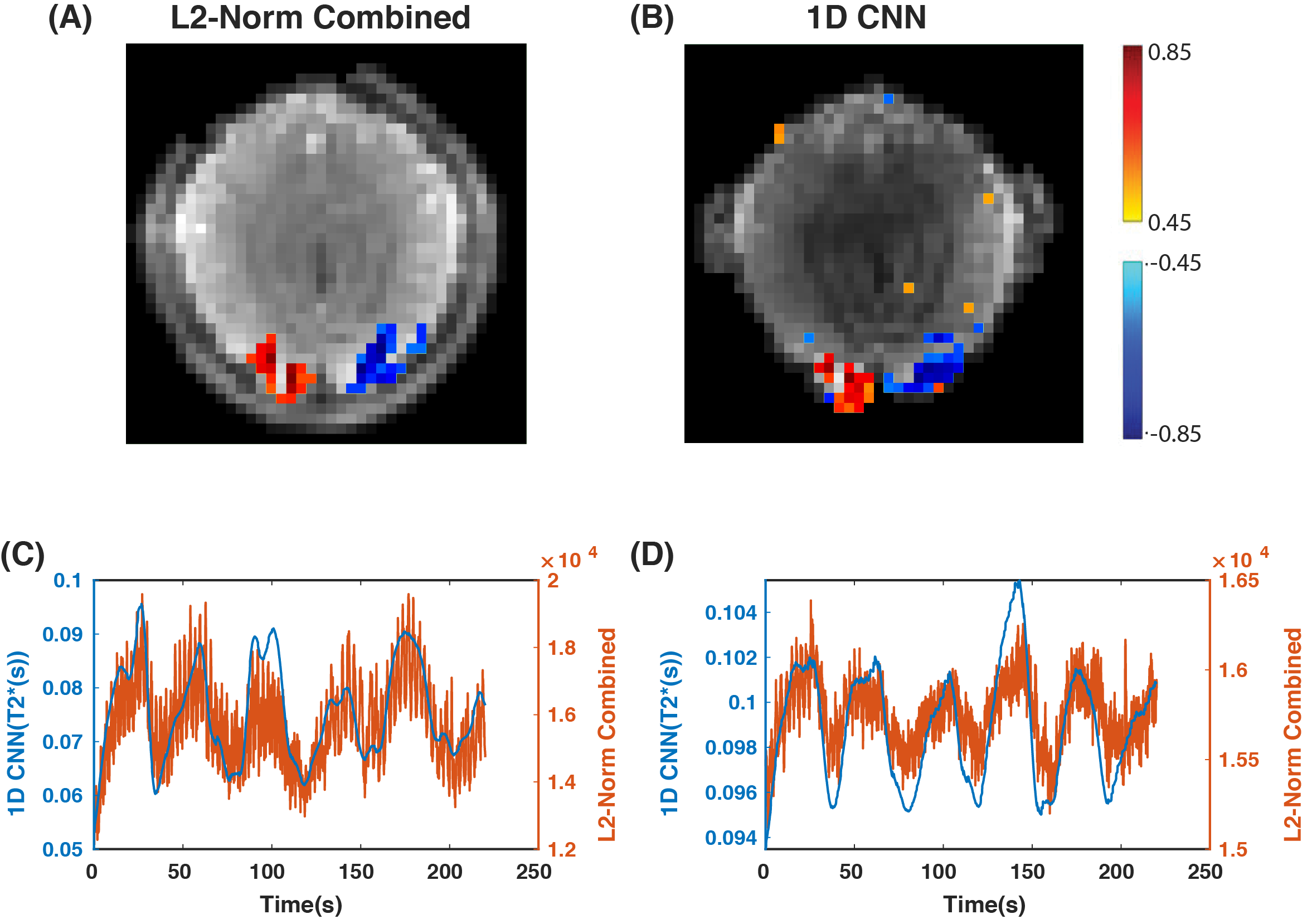
Fig.5A-B shows the 1DCNN and $$$L_2$$$-norm combined activation maps. The overall spatial structure of the brain is preserved in the $$$T_2^*$$$-weighted image derived from the 1DCNN, and the activations are clustered in the visual area of the cortex. This result is comparable to the activations in the $$$L_2$$$-norm combined image of the brain.
Fig.5C-D shows two different time courses from two activated pixels. The 1DCNN time courses are smoother with less respiration induced fluctuations and thermal noise compared to the $$$L_2$$$-norm combined time courses.
Discussion and Conclusion
In this study, we proposed using a 1DCNN for OSSI signal combination to solve the frequency sensitivity issues associated with the $$$L_2$$$-norm combined signals by directly estimating the BOLD signal from the OSSI signal. We were able to use this method to reduce thermal and respiratory induced noise in data from simulations and human subjects. However, the 1DCNN overestimates the $$$T_2^*$$$ values in human subject data as seen in the time courses from Fig.5C-D.Moving forward, we plan to explore this issue by examining different normalization techniques for the training data and optimizing our network architecture.
Acknowledgements
We wish to acknowledge the support of NIH Grant U01EB026977.References
[1] Miller, Karla L. "FMRI using balanced steady-state free precession (SSFP)." Neuroimage 62.2 (2012): 713-719.
[2] Guo, Shouchang, and Douglas C. Noll. "Oscillating steady‐state imaging (OSSI): A novel method for functional MRI." Magnetic Resonance in Medicine 84.2 (2020): 698-712.
[3] Friston, Karl J., Peter Jezzard, and Robert Turner. "Analysis of functional MRI time‐series." Human brain mapping 1.2 (1994): 153-171.
[4] Cao, Amos A., and Douglas C. Noll. "A retrospective physiological noise correction method for oscillating steady‐state imaging." Magnetic Resonance in Medicine 85.2 (2020): 936-944.
Figures
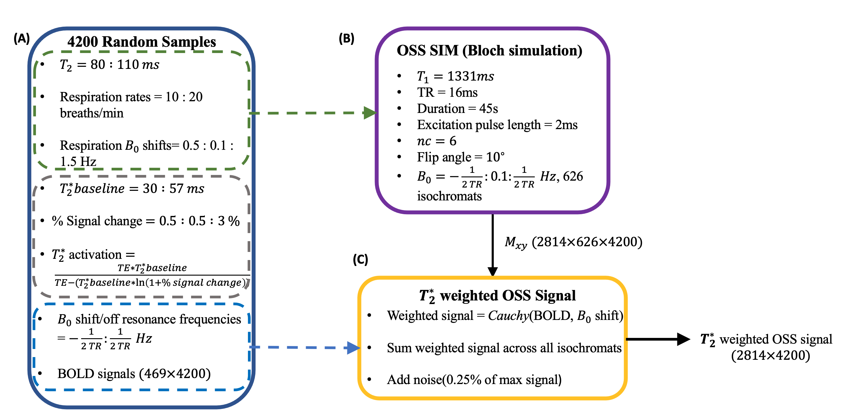
Fig. 1. A-shows parameters that were sampled using Monte Carlo simulation, and the range of values from which these parameters were sampled. 4200 different BOLD trajectories were generated by weighing the BOLD responses with different T2* activation and baseline values.
B-shows the static simulation parameters for generating OSSI signals that are corrupted by different amount of respiration.
C-the final signal produces a T2*-weighted OSSI signal corrupted by thermal and respiratory induced noise.
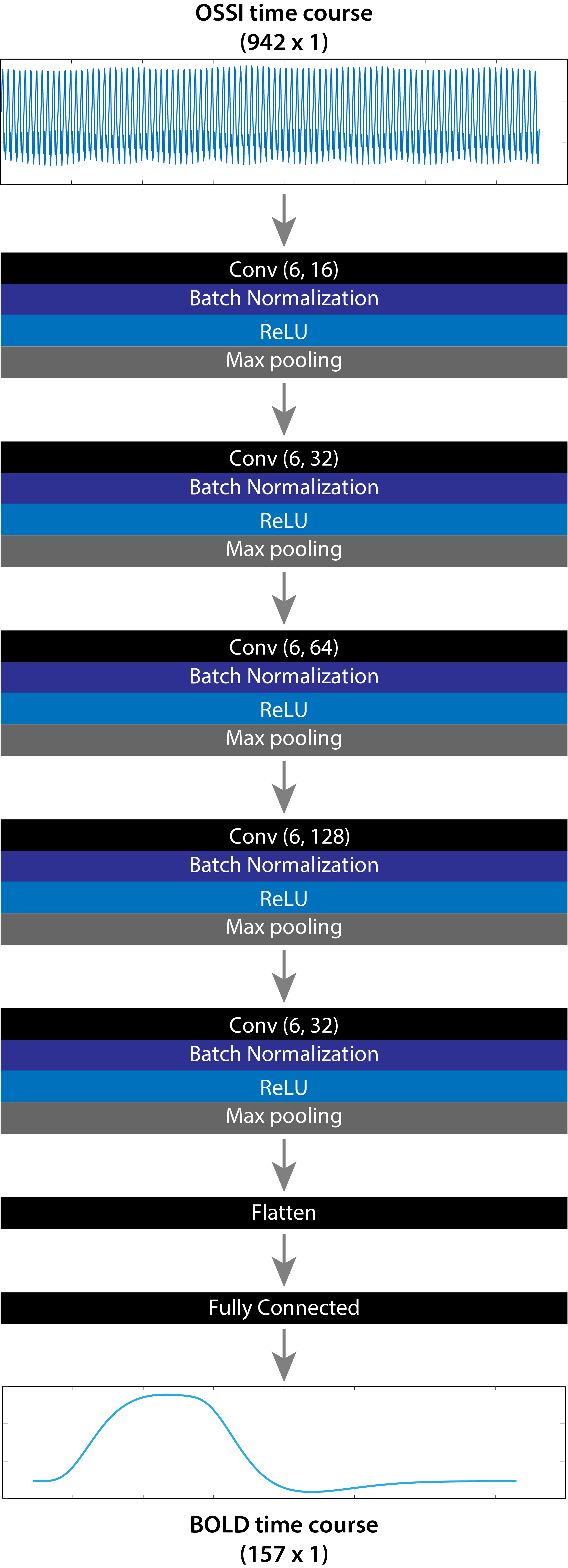
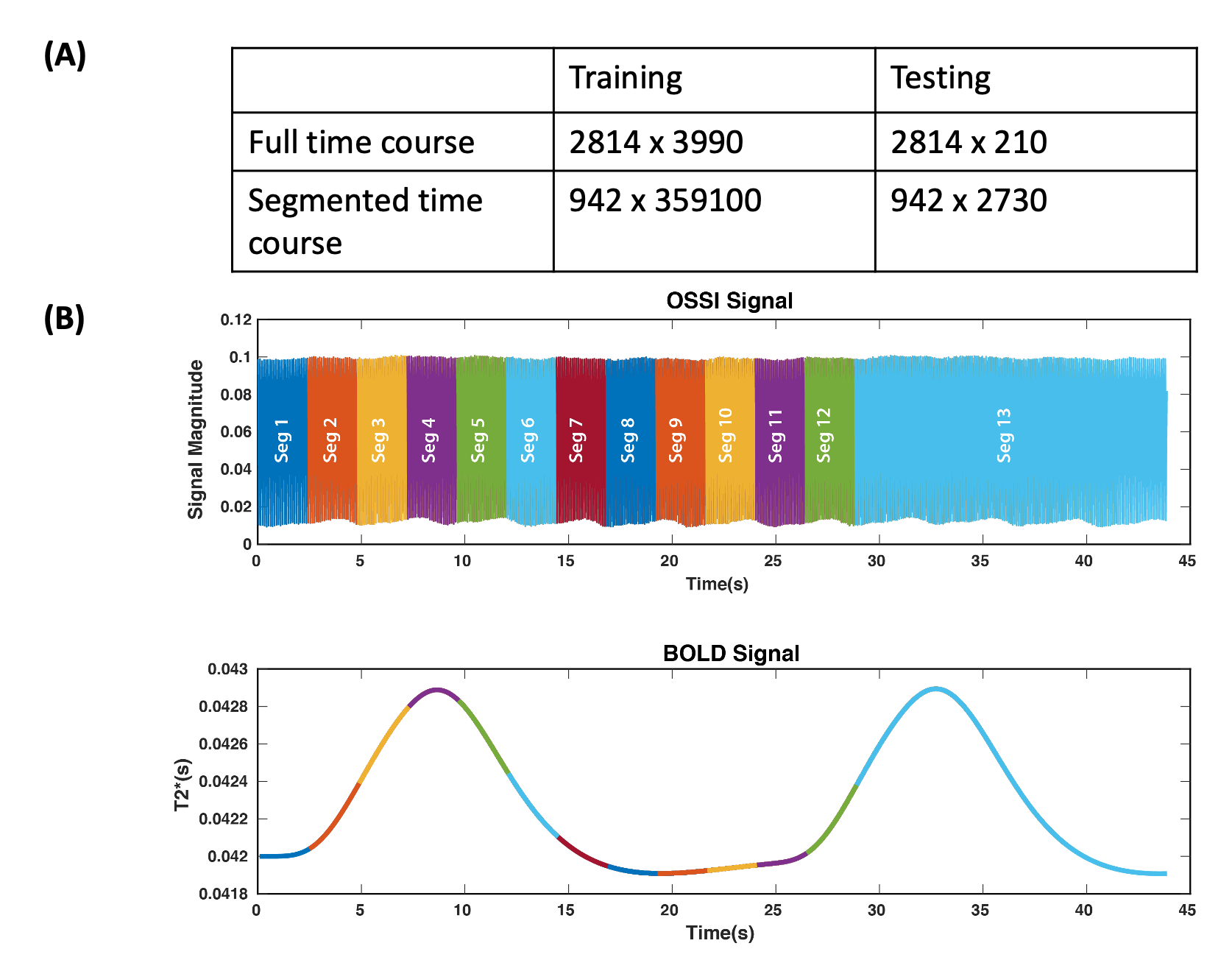
Fig. 3. A-For training, each full OSSI time course was divided into 90 random 15s segments.
For testing, we divided each OSSI time course from the test samples into 13 consecutive and overlapping 15s segments, as shown in B. The 1DCNN outputs were stitched back to form the original 45s long BOLD signal using a Hann weighting function of the overlapping segments.
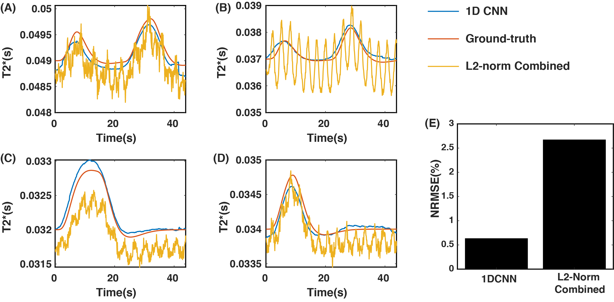
Fig. 4. Simulation Result: A-D Compares BOLD time courses for both methods. E compares NRMSE for both methods.