2674
Creating a robust BOLD fMRI phantom using microspheres: How well do microspheres approximate microvasculature?1Rotman Research Institute, Baycrest Health Sciences, North York, ON, Canada, 2A. A. Martinos Center for Biomedical Imaging, Harvard Medical School, Massachusetts General Hospital, Boston, MA, United States, 3Department of Medical Biophysics, University of Toronto, Toronto, ON, Canada
Synopsis
BOLD phantoms are important for the evaluation of fMRI acquisition techniques, but validating numerical simulations based on conventional random-cylinder models of the microvasculature is difficult because available phantoms lack the microstructure required to emulate these geometries. In comparison, a phantom using randomly positioned microspheres is a more feasible alternative, but it is still unclear how well microspheres approximate cylinders in their transverse relaxation behaviour. In this work, we use 3D Monte Carlo simulations to compare the behaviour of the two perturber types at 3 T.
Introduction
BOLD phantoms can be an important tool for validating the contrast mechanisms and signal sources fMRI acquisitions, including gas-free calibrated fMRI, vascular fingerprinting 1–3 and in investigating the microvascular specificity of fMRI acquisitions 4. Due to the common use of the infinite cylinder model to approximate microvasculature 5, previous BOLD phantoms have been built using microscopic strings 4,6. However, the orientation distribution and density of such strings can be difficult to manipulate accurately, and microspheres have been proposed as a viable alternative 7,8. Microsphere-based phantoms have been used successfully to generate BOLD-like signal behaviour 8. Nonetheless, it is unclear how closely microspheres can approximate the behaviour of the microvasculature (cylinders) assumed in most numerical modelling approaches. To test the appropriateness of these available microsphere phantoms to BOLD simulations, in this work we use 3D Monte Carlo simulations to explicitly compare the transverse relaxation of the infinite-cylinder and microsphere models at 3 T.Methods
All steps are implemented as custom scripts in Python. We generate a 3D voxel of randomly oriented and uniformly distributed infinite cylinders following the methods of Martindale et al. 9. For spherical perturbers, positions are uniformly sampled within the cubic voxel space. The volumes of both cylinders and spheres are calculated analytically and cumulatively to reach the desired perturber volume fractions (set to the target values of realistic cerebral-blood volume (CBV) fractions).The BOLD signal is modeled as extravascular Monte Carlo spin diffusion similar to Ogawa et al. 5. Both the cylindrical and spherical perturbers’ magnetic field offsets (ΔB) are calculated analytically as a function of spin position 9. The Larmor equation is then used to convert this offset to an off-resonance. We assume a B0 of 3 T and ignore intrinsic T2 relaxation.
Molecular diffusion is implemented using Monte Carlo simulations with 5000 spins randomly positioned outside the vessels. These spins are allowed to diffuse in the extravascular space using Einstein’s method at a diffusion coefficient of 1 μm2/ms. The mean dephasing of all spins at each timestep (dt = 0.2 ms), in combination with the specific pulse sequence, results in the desired BOLD signal. The reversible transverse relaxation rate (R2’) is finally calculated from the exponential decay model. We do so for gradient-echo (GE), spin-echo (SE) and asymmetric spin-echo (ASE) contrast. The target echo times are 30ms for GE, 70ms for SE and 70ms for ASE. For ASE, the time shift τ is 50ms. From these results, we also approximate the value of the BOLD model parameter β, which characterizes the dependence of R2’ on susceptibility, i.e. β=ln(dR2’)/ln(dχ), which is known to vary with perturber radius and field strength 10,11.
Results
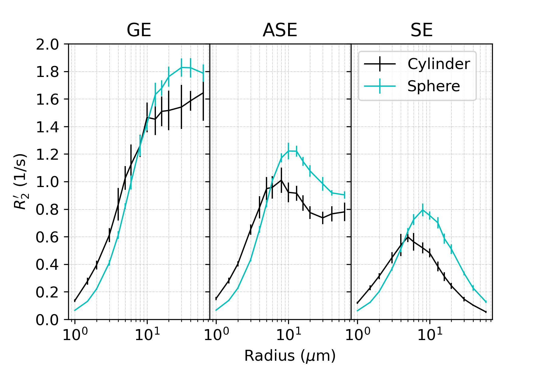
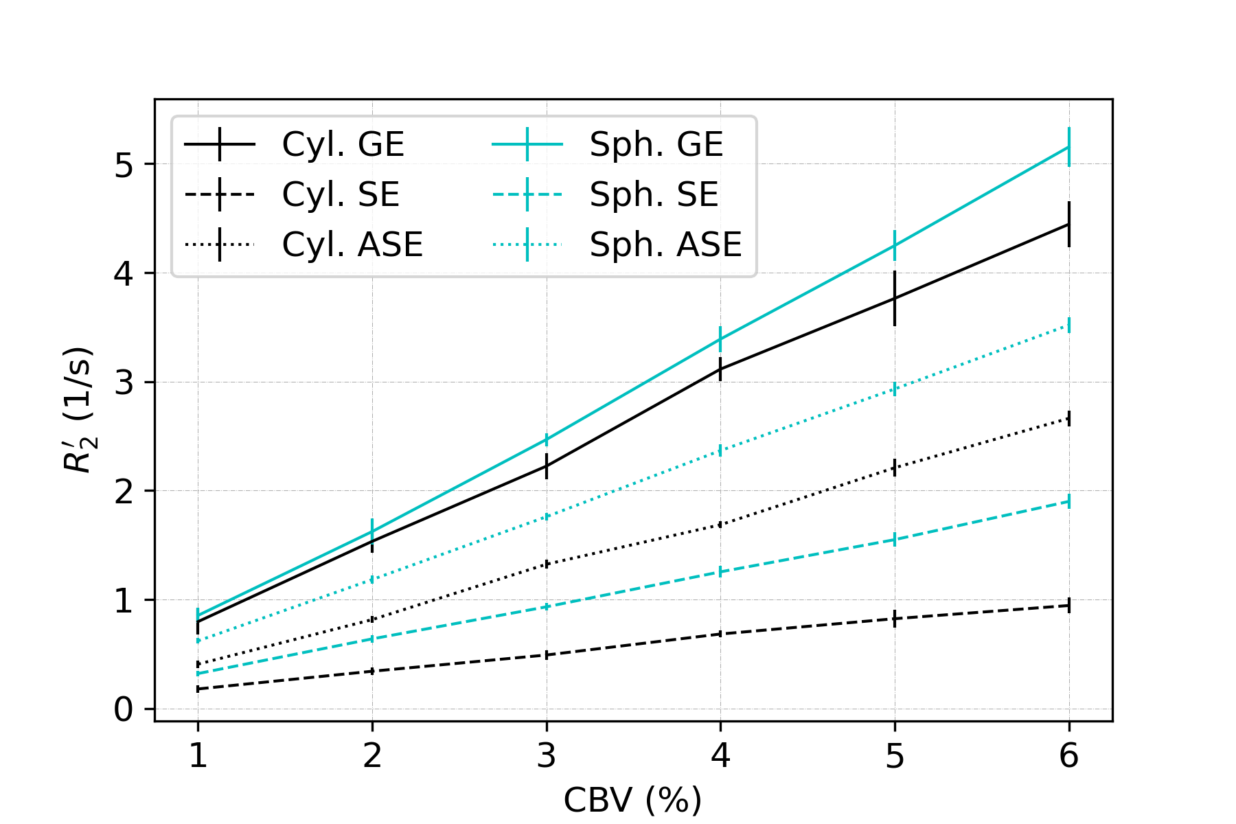
In all figures, data points are the mean of simulations over 10 iterations of vessel networks with the standard deviation shown by error bars. In Figure 1, we show R2’ vs. vessel radius plots for all pulse sequences, demonstrating that both spherical and cylindrical perturbers result in R2’ plateaus for GE and peaks for SE and ASE, similar to those reported by Boxerman et al. 12. However, it also is observed that for small radii, R2’ values of cylindrical perturbers are initially higher than those of spheres at equivalent radius, but are surpassed by them at higher radii. This crossover point depends on the sequence used but falls in the range of ~4-8 μm for the parameters explored here.Figure 2 shows that both perturber types result in a linear R2’ dependence on CBV. However, for radii less than the crossover point mentioned above, the slopes for spheres are shallower than for cylinders (results not shown).
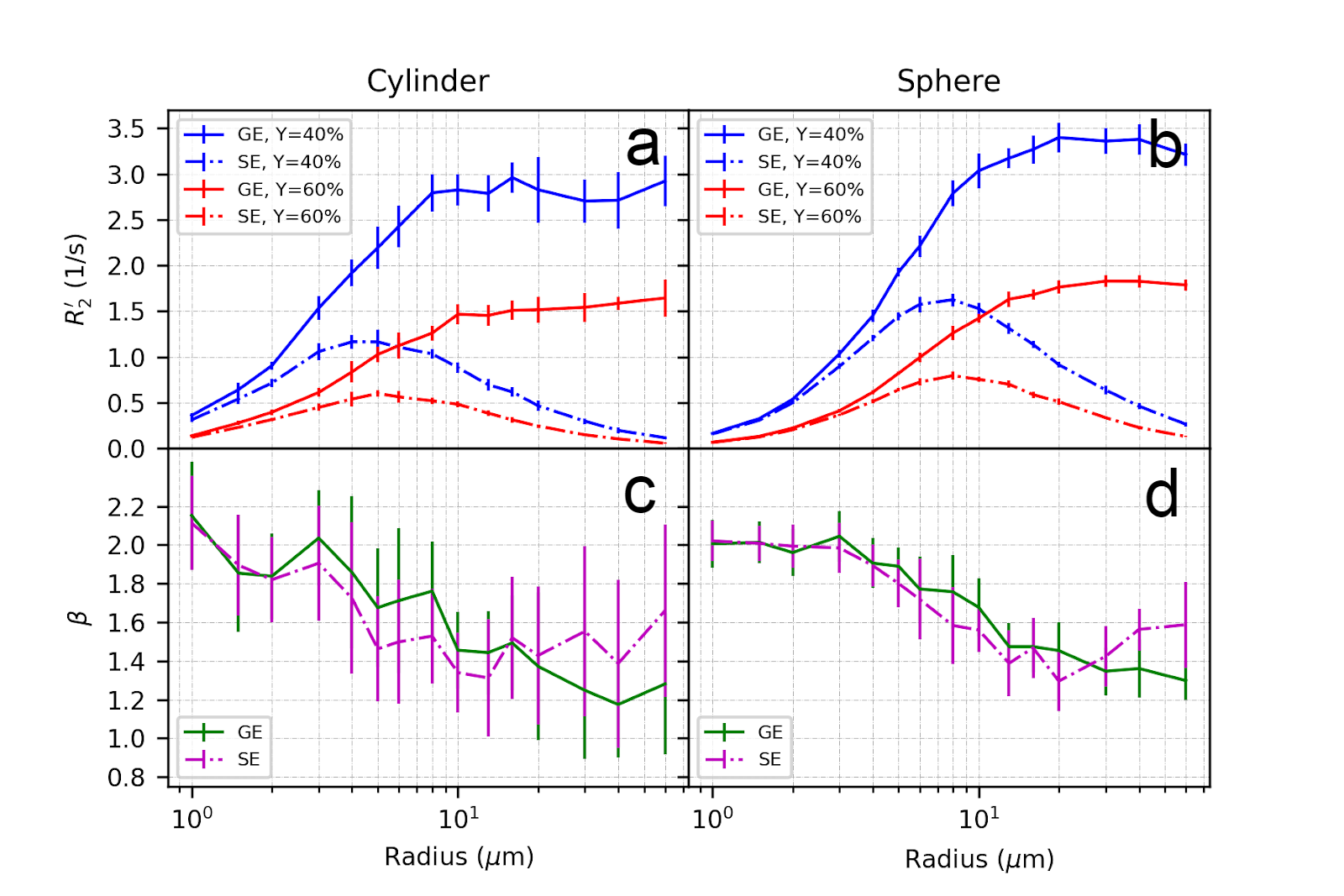
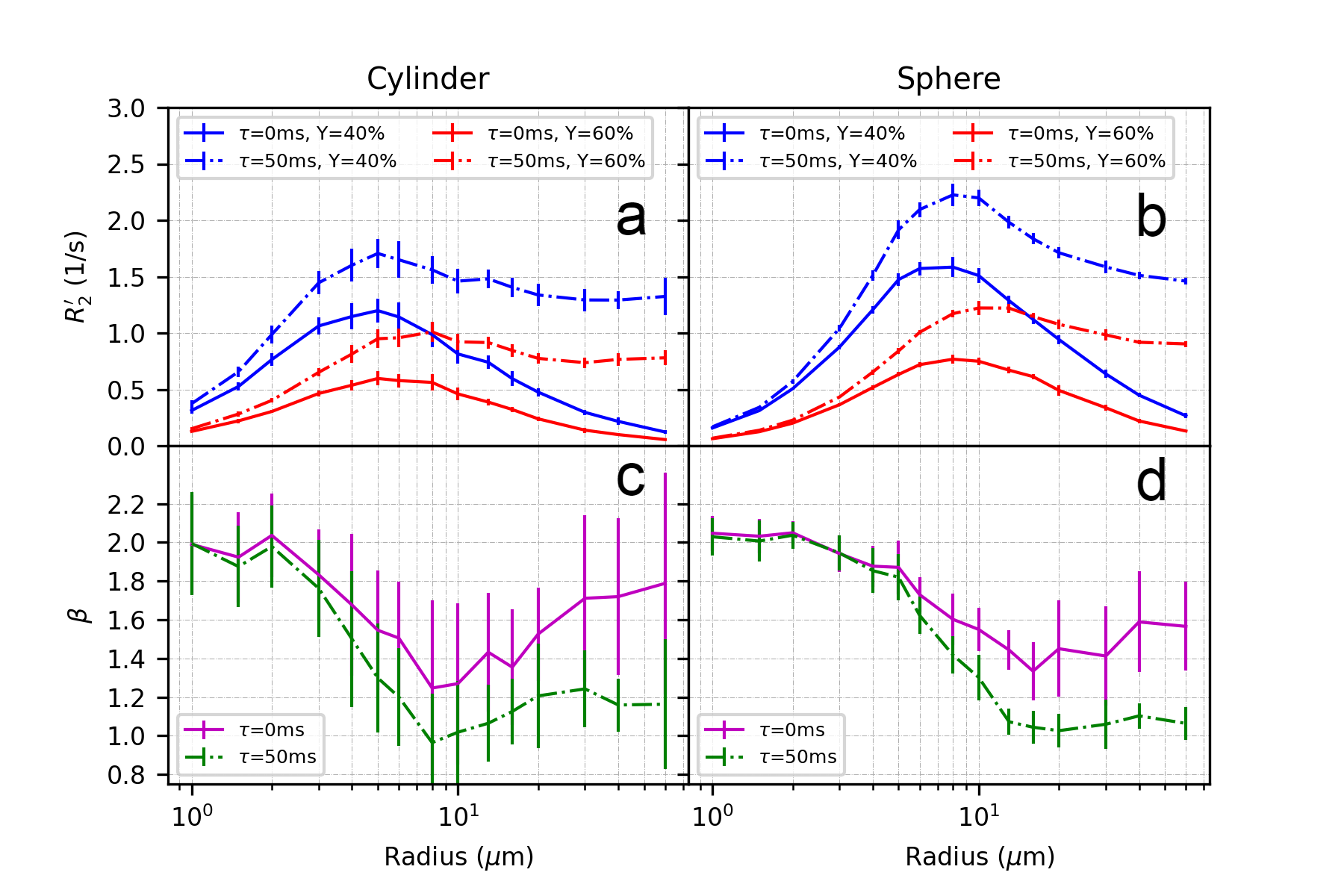
Figure 3 and Figure 4 illustrate the effect of blood oxygenation (Y) on the R2’-radius relationship for GE, SE and ASE. We chose Y1 = 40%, Y2 = 60%, and in all cases, R2’ increases with Y decrease 5. We calculate β, with each Δχ associated with Y. For both spheres and cylinders, β approaches 2 at small radii. For GE, β approaches 1 at larger radii, whereas for SE and ASE, β is minimum around 10 μm for cylinders and 20 μm for spheres, and increases thereafter.
Discussion
In this work, using 3D Monte Carlo BOLD simulations at 3 T, we demonstrate that when all parameters are matched, microspherical perturbers demonstrate a somewhat exaggerated but similarly behaved version of the cylindrical R2’ dependence on perturber radius, CBV and Y. This may be the result of the extravascular off-resonance effects having a cubic dependence with spheres and square dependence with cylinders. Nonetheless, it is clear that microspherical perturbers can indeed approximate the behaviour of infinite cylinders. This finding lays the theoretical foundation for using microspheres to simulate microvasculature in phantom studies, and for calibrating the results to reflect the behaviour of cylindrical vessels.Acknowledgements
We thank the Canadian Institutes for Health Research (CIHR) (grant MFE-164755 and grant FRN# 148398), the Natural Sciences and Engineering Research Council of Canada (NSERC) (grant FGPIN# 418443) and National Institues of Health (NIH) (NIMH grant R01-MH111419 and NIBIB grant R01-EB019437) for financial support.References
1. Blockley, N. P., Griffeth, V. E. M., Simon, A. B., Dubowitz, D. J. & Buxton, R. B. Calibrating the BOLD response without administering gases: comparison of hypercapnia calibration with calibration using an asymmetric spin echo. Neuroimage 104, 423–429 (2015).
2. Christen, T. et al. MR vascular fingerprinting: A new approach to compute cerebral blood volume, mean vessel radius, and oxygenation maps in the human brain. Neuroimage 89, 262–270 (2014).
3. Berman, A. J. L. et al. Gas-free calibrated fMRI with a correction for vessel-size sensitivity. Neuroimage 169, 176–188 (2018).
4. Pannetier, N. A., Sohlin, M. & Christen, T. Numerical modeling of susceptibility‐related MR signal dephasing with vessel size measurement: Phantom validation at 3T. Magnetic resonance (2014).
5. Ogawa, S. et al. Functional brain mapping by blood oxygenation level-dependent contrast magnetic resonance imaging. A comparison of signal characteristics with a biophysical model. Biophys. J. 64, 803–812 (1993).
6. Sedlacik, J. & Reichenbach, J. R. Validation of quantitative estimation of tissue oxygen extraction fraction and deoxygenated blood volume fraction in phantom and in vivo experiments by using MRI. Magn. Reson. Med. 63, 910–921 (2010).
7. Weisskoff, R. M., Zuo, C. S., Boxerman, J. L. & Rosen, B. R. Microscopic susceptibility variation and transverse relaxation: theory and experiment. 31, 601–610 (1994).
8. Scheffler, K., Heule, R., G Báez-Yánez, M., Kardatzki, B. & Lohmann, G. The BOLD sensitivity of rapid steady-state sequences. Magn. Reson. Med. (2018) doi:10.1002/mrm.27585.
9. Martindale, J., Kennerley, A. J., Johnston, D., Zheng, Y. & Mayhew, J. E. Theory and generalization of Monte Carlo models of the BOLD signal source. Magn. Reson. Med. 59, 607–618 (2008).
10. Griffeth, V. E. M. & Buxton, R. B. A theoretical framework for estimating cerebral oxygen metabolism changes using the calibrated-BOLD method: Modeling the effects of blood volume distribution, hematocrit, oxygen extraction fraction, and tissue signal properties on the BOLD signal. NeuroImage vol. 58 198–212 (2011).
11. Croal, P. L., Driver, I. D., Francis, S. T. & Gowland, P. A. Field strength dependence of grey matter R2* on venous oxygenation. NeuroImage vol. 146 327–332 (2017).
12. Boxerman, J. L., Hamberg, L. M., Rosen, B. R. & Weisskoff, R. M. MR contrast due to intravascular magnetic susceptibility perturbations. Magn. Reson. Med. 34, 555–566 (1995).
Figures