2655
Improving automated aneurysm detection on multi-site MRA data: lessons learnt from a public machine learning challenge1Department of Radiology, Lausanne University Hospital and University of Lausanne, Lausanne, Switzerland, 2Center for Psychiatric Neuroscience, Lausanne University Hospital and University of Lausanne, Lausanne, Switzerland, 3Medical Image Analysis Laboratory (MIAL), Centre d’Imagerie BioMédicale (CIBM), Lausanne, Switzerland
Synopsis
Machine learning challenges serve as a benchmark for determining state-of-the-art results in medical imaging. They provide direct comparisons between algorithms, and realistic estimates of generalization capability. By participating in the Aneurysm Detection And segMentation (ADAM) challenge, we learnt the most effective deep learning design choices to adopt when tackling automated brain aneurysm detection on multi-site data. Adjusting patch overlap ratio during inference, using a hybrid loss, resampling to uniform voxel spacing, using a 3D neural network architecture, and correcting for bias field were the most effective. We show that, when adopting these expedients, our model drastically improves detection performances.
1 - Introduction
The task of brain aneurysm detection in Magnetic Resonance Angiography (MRA) has been extensively studied in past years1-4. Although these novel methods showed encouraging results, they were tested on in-house datasets, which makes fair comparison nearly impossible. In addition, some of them2,4 applied their algorithms on Maximum Intensity Projection (MIP) images, rather than on MRA. At MICCAI 2020, the first public challenge on aneurysm detection in MRA was organized (ADAM5). This represented a turning point since it finally provided an unbiased comparison between research groups. To have a realistic idea of how our model generalized to unseen data from another hospital, we decided to participate. This work describes the model that we initially submitted to the challenge; then, it illustrates the beneficial impact of the winning trends on our network. Lastly, it shows the domain gap in performances across different sites.2 - Materials and Methods
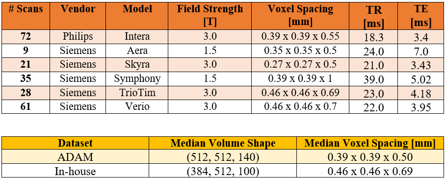
2.1 DataThe training data was composed of both ADAM (challenge) and in-house data. For ADAM, 113 subjects presenting a total of 125 aneurysms were provided. The annotations of all challenge data were manually drawn slice by slice in the axial plane by two trained radiologists. Instead, the in-house data consisted of 212 subjects who underwent clinically-indicated MRA in our hospital, and presented a total of 110 aneurysms. Patients were scanned using a 3D gradient recalled echo sequence with Partial Fourier technique (details in Figure 1). For all our subjects, coarse manual masks (spheres enclosing the aneurysms) were drawn around aneurysms by one radiologist with 3+ years of experience in neuroimaging.
To assess the gap in performances across different sites, evaluation was performed both on the ADAM test set (141 subjects, unreleased) and on 38 new in-house patients presenting 44 aneurysms. When evaluating on the ADAM test set, we trained the network with a combination of our in-house data and the ADAM training set. Similarly, when evaluating on our in-house test set, we trained the model with all ADAM data and our training set.
2.2 First challenge submission
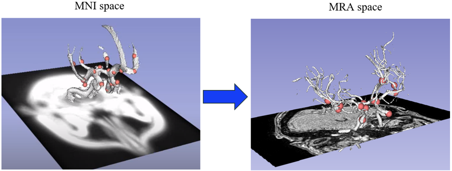
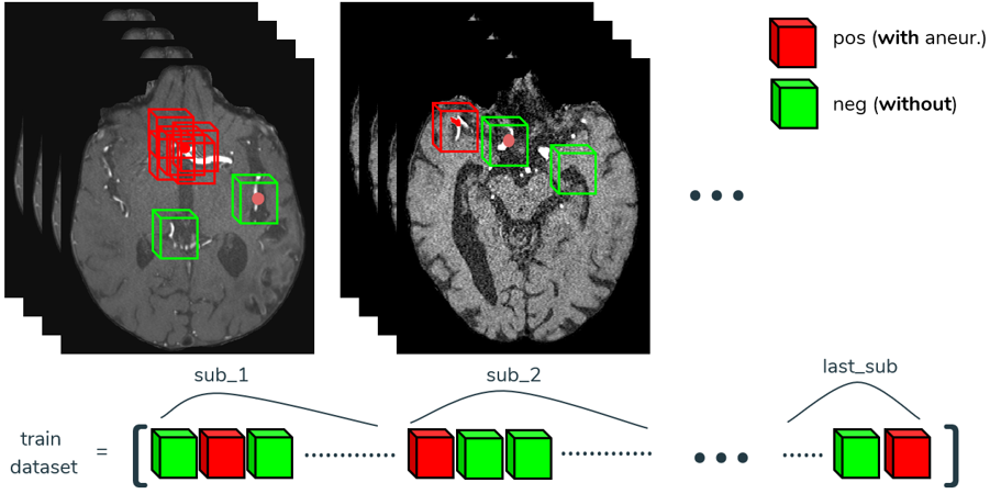
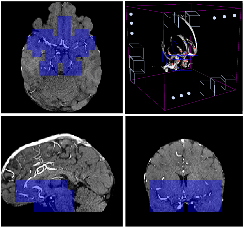
Here, we describe our first method. Two preprocessing steps were applied: first, we performed brain extraction on all volumes with FSL-BET6; then, we co-registered a probabilistic vessel atlas7 from MNI space to the MRA space of each subject using ANTS8. Furthermore, one of our radiologists pinpointed in MNI space the location of 24 landmark points where aneurysm occurrence is most frequent, and we also co-registered these points to individual MRA space (Figure 2). The training dataset was composed of 3D patches extracted from the skull-stripped MRA volumes (patch selection details in Figure 3). To reduce class imbalance, we applied 6 augmentation techniques on patches containing aneurysms, namely horizontal and vertical flipping, rotations, and contrast adjustment. As deep learning model, we implemented a 3D-UNET9 in Tensorflow 2.1. This was initialized with the Xavier method10 and trained for 500 epochs with adaptive learning rate, Adam11 optimizer and dice loss12, on a GeForce RTX 2080TI with 11GB of SDRAM. At inference, patient-wise detection was performed with a sliding-window approach, without patch overlapping. Only patches which are both within a minimum distance from the landmark points and have an average brightness higher than a specific threshold were retained. The rationale behind this choice was to only focus on patches located in the Willis polygon (Figure 4). The probabilistic segmentation output was binarized with an empirical threshold (0.75). Then, only the largest connected component was retained for each patch, and its center-of-mass was used as aneurysm center location.
2.3 Post-challenge submission
The model that we later re-submitted was based on the one above, but it was modified with the winning trends adopted by the top-performing teams which were:
- Sliding-window overlapping: we increased patch overlap during inference to 25%.
- Loss function: we used a combination of cross-entropy and Dice as in 13 (with $\alpha=0.5$), instead of plain Dice.
- Resampling: since both our dataset and the challenge dataset contain images acquired with different parameters (see lower table in Figure 1), resampling to a uniform voxel spacing mitigates site differences.
- Bias-field correction: removing smooth low-frequency noise alleviates part of the inter-site and inter-subject intensity variabilities.
3 - Results
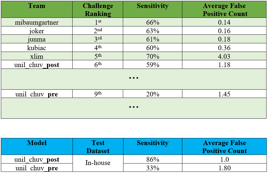
Figure 5 illustrates all detection results both for the two challenge submissions and for our in-house test set. With the modified network, we improved our detection ranking from 9th to 6th position. Moreover, there was a drastic sensitivity increase (+39% on ADAM, +53% on in-house), as well as a slight reduction in average false positive count on both datasets. Lastly, we noticed a substantial drop in performances across sites (in-house sensitivity=86% vs. challenge sensitivity=59%).4 - Discussion
We believe the challenge brought two main contributions: on one hand, it provided the first unbiased comparison of detection models for MRA data; on the other hand, it outlined the most efficient experimental choices for achieving state-of-the-art results. Overall, domain gaps due to site differences still represent an obstacle for effectively applying machine learning techniques on clinical data. However, challenges offer a precious feedback mechanism to push the field forward.Acknowledgements
We would like to thank the challenge organizing team, and especially the main organizer Kimberley Timmins who kindly recomputed the results of our second submission.
References
1. Ueda, Daiju, et al. “Deep learning for MR angiography: automated detection of cerebral aneurysms.” Radiology 290.1 (2019): 187-194.
2. Stember, Joseph N., et al. “Convolutional neural networks for the detection and measurement of cerebral aneurysms on magnetic resonance angiography.” Journal of digital imaging 32.5 (2019): 808-815.
3. Sichtermann, T., et al. “Deep Learning–Based Detection of Intracranial Aneurysms in 3D TOF-MRA.” American Journal of Neuroradiology 40.1 (2019): 25-32.
4. Nakao, Takahiro, et al. “Deep neural network‐based computer‐assisted detection of cerebral aneurysms in MR angiography.” Journal of Magnetic Resonance Imaging 47.4 (2018): 948-953.
5. Kimberley Timmins, Edwin Bennink, Irene van der Schaaf, Birgitta Velthuis, Ynte Ruigrok, & Hugo Kuijf. (2020, March 19). Intracranial Aneurysm Detection and Segmentation Challenge. Presented at the 23rd International Conference on Medical Image Computing and Computer Assisted Intervention (MICCAI 2020), Lima, Peru: Zenodo. http://doi.org/10.5281/zenodo.3715848
6. Smith, S. M. (2002). “Fast robust automated brain extraction.” Human brain mapping, 17(3), 143-155.
7. Mouches, Pauline, and Nils D. Forkert. “A statistical atlas of cerebral arteries generated using multi-center MRA datasets from healthy subjects.” Scientific data 6.1 (2019): 1-8.
8. Avants, Brian B., et al. “A reproducible evaluation of ANTs similarity metric performance in brain image registration.” Neuroimage 54.3 (2011): 2033-2044.
9. Çiçek, Özgün, et al. “3D U-Net: learning dense volumetric segmentation from sparse annotation.” International conference on medical image computing and computer-assisted intervention. Springer, Cham, 2016.
10. Glorot, Xavier, and Yoshua Bengio. “Understanding the difficulty of training deep feedforward neural networks.” Proceedings of the thirteenth international conference on artificial intelligence and statistics. 2010.
11. Kingma, Diederik P., and Jimmy Ba. “Adam: A method for stochastic optimization.” arXiv preprint arXiv:1412.6980 (2014).
12. Milletari, Fausto, Nassir Navab, and Seyed-Ahmad Ahmadi. “V-net: Fully convolutional neural networks for volumetric medical image segmentation.” 2016 fourth international conference on 3D vision (3DV). IEEE, 2016.
13. Taghanaki, Saeid Asgari, et al. “Combo loss: Handling input and output imbalance in multi-organ segmentation.” Computerized Medical Imaging and Graphics 75 (2019): 24-33.
Figures