2610
QTI+: a constrained estimation framework for q-space trajectory imaging1Dept. of Mathematics, Linköping University, Linköping, Sweden, 2Dept.of Computer Science, University of Copenhagen, Copenhagen, Denmark, 3Dept. of Biomedical Engineering, Linköping University, Linköping, Sweden, 4Center for Medical Image Science and Visualization, Linköping University, Linköping, Sweden, 5Department of Applied Mathematics and Computer Science, Technical University of Denmark, Lyngby, Denmark, 6Laboratory for Mathematics in Imaging, Department of Radiology, Brigham and Women’s Hospital, Harvard Medical School, Boston, Boston, MA, United States
Synopsis
Q-space trajectory imaging (QTI) provides a means to estimate the moments for a diffusion tensor distribution (DTD) characterizing the tissue. Commonly employed estimation methods do not typically yield mathematically acceptable estimates, namely that the tensor distribution consists of symmetric positive semidefinite tensors and that the second cumulant represents a covariance. We introduce the QTI+ framework, which utilizes semi-definite programming (SDP) to address this issue. Simulations using a DTD taking the form of a non-central Wishart distribution as well as real data show a marked improvement in the technique's robustness to noise compared to more common (unconstrained) estimation methods.
Introduction
Diffusion encoding via gradient waveforms with a time-dependent gradient orientation1 has advanced our ability to characterize the intravoxel tissue structure. Notably, q-space trajectory imaging (QTI)2 enables the estimation of new scalar measures indicating the microscopic and macroscopic anisotropies, size variance, and orientational coherence associated with the tissue make-up through the indices $$$C_\mu=\mu\phantom{}FA^2,C_M=FA^2,C_{MD}$$$, and $$$C_C$$$, respectively. This is accomplished under the assumption of a diffusion tensor distribution (DTD) representing the tissue microstructure3, in which case the influence of the gradient waveform is fully captured by the second order B-tensor4. QTI exploits the sensitivity of the diffusion signal to the statistical moments of the parameters describing each microdomain5. In fact, the clinically-relevant low b-value ($$$b=Tr(B_{ij})=B_{ii}$$$) regime of the signal was shown2 to be described solely by the second-order mean ($$$\hat{D}_{ij}$$$) and fourth-order covariance tensors ($$$C_{ijkl}$$$) of the DTD through the relationships$$S\approx\phantom{}S_0e^{–B_{ij}\hat{D}_{ij}+B_{ij}B_{kl}C_{ijkl}}\mbox{ or }\log\phantom{}S\approx\log S_0–B_{ij}\hat{D}_{ij}+B_{ij}B_{kl}C_{ijkl}.
$$The key step in obtaining the mentioned scalar measures involves finding acceptable estimates of the two tensors. The first equation above lends itself to a non-linear least square problem (NLLS). After correction for heteroscedasticity, the second expression gives a weigted linear least squares problem (WLLS) of the form $$$\mathbf{A}\mathbf{x}=\mathbf{b}$$$. Should $$$\mathbf{A}$$$ be rank deficient, it is customary to employ subspace methods (WLLS(ss)) in QTI's common practice6. Here, we introduce the QTI+ framework that enforces mathematically necessary conditions on the estimates and demonstrate the superiority of this approach over the commonly-employed estimation methods WLLS/WLLS(ss).
Methods
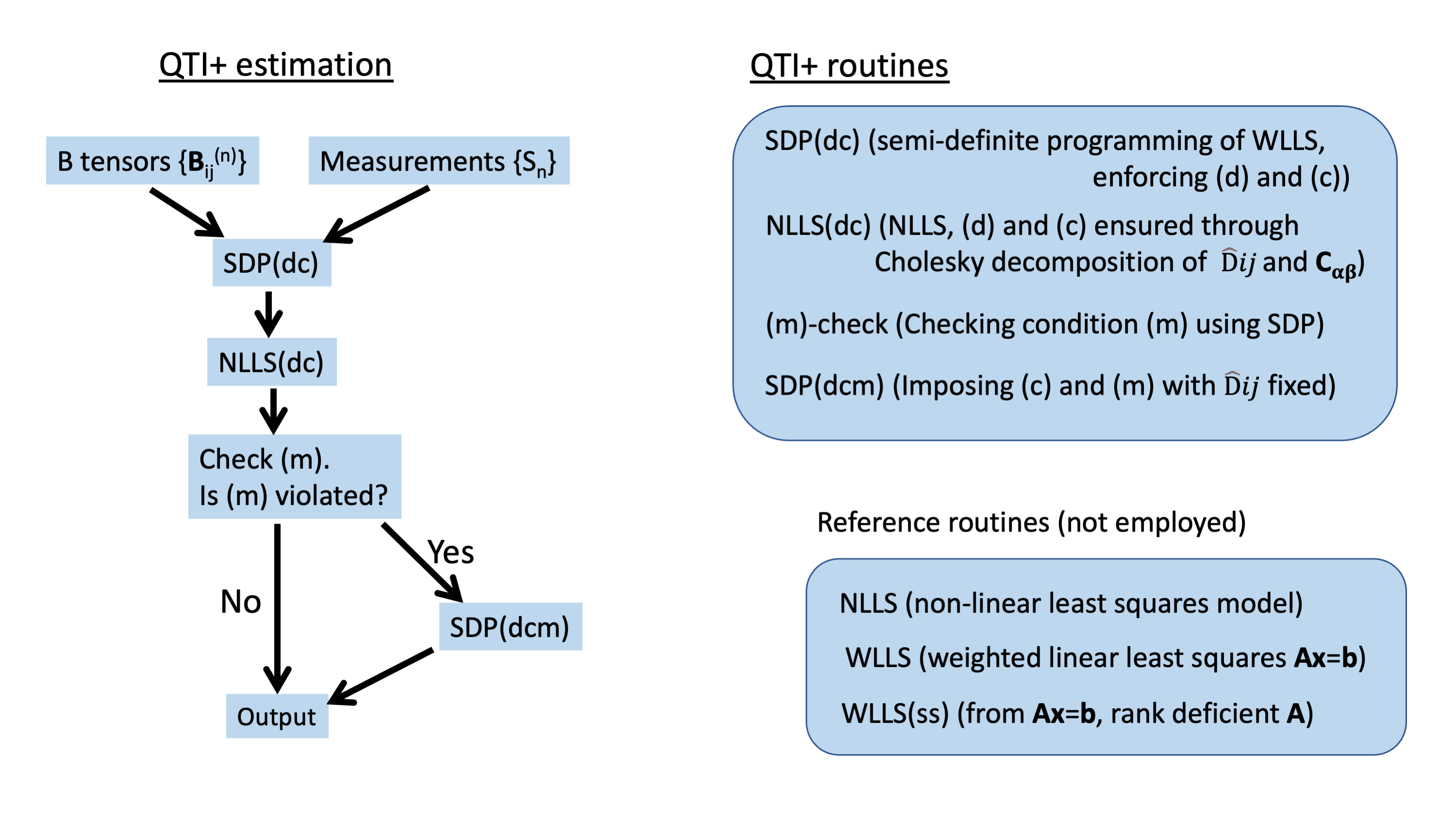
The frameworkWe identified three (necessary but not sufficient) independent conditions that every DTD has to obey
(d) $$$\hat D_{ij}\succeq\phantom{}0$$$, (in this work $$$\succeq\phantom{}0$$$ indicates the symmetric matrix being positive semi-definite)
(c) $$$C_{\alpha\beta}\succeq\phantom{}0$$$, (where $$$C_{\alpha\beta}$$$ is a $$$6\times\phantom{}6$$$ representation of $$$C_{ijkl}$$$ in a suitable basis)
(m) $$$M_{ijkl}u_iu_jv_kv_l\geq\phantom{}0$$$ for all vectors $$$u_i$$$ and $$$v_i$$$, where $$$M_{ijkl}=C_{ijkl}+\hat{D}_{ij}\hat{D}_{kl}$$$ is the second moment tensor.
We devised a framework consisting of four optimization problems that could be employed in synergy to provide estimates that guarantee the conditions above. The overall framework is depicted in Figure 1. Similar to the approach taken in the introduction of other ´+` methods7 for signal representations8-11 employed for single diffusion encoding experiments, our scheme employs semidefinite programming (SDP) to introduce hard constraints to the estimation.
Simulations
We performed simulations of DTDs distributed according to a non-central Wishart distribution for which the signal12,13, mean and covariance tensors are given by
$$
\begin{align}
E(\mathbf{B})=\ &|\mathbf I + \mathbf{\Sigma}\mathbf{B}|^{-p}\exp(-\mathrm{Tr}[\mathbf{B}(\mathbf{I}+ \mathbf{\Sigma}\mathbf{B})^{-1}\mathbf{\Omega} ] ) \quad\mbox{(subscripts dropped for brevity)}\\
\widehat{D}_{ij}=\ & p\Sigma_{ij}+\Omega_{ij} \\
C_{ijk\ell}=\ & \frac{p}{2}(\Sigma_{i\ell}\Sigma_{jk}+\Sigma_{ik}\Sigma_{j\ell}) +\frac{1}{2}(\Sigma_{jk}\Omega_{i\ell}+\Sigma_{i\ell}\Omega_{jk}+\Sigma_{j\ell}\Omega_{ik}+\Sigma_{ik}\Omega_{j\ell}) \ ,
\end{align}
$$where $$$p$$$ is the shape parameter, $$$\Sigma_{ij}$$$ the scale matrix and $$$\Omega_{ij}$$$ is the noncentrality matrix. In our experiments we set $$$\Sigma_{ij}=\hat D_{ij}/(5p)$$$. One simulation featured $$$p=2$$$ and an isotropic $$$\hat D_{ij}$$$ with $$$1/3Tr(\hat D_{ij})$$$=0.7$$$\mu$$$m$$$^2$$$/ms, while the second simulation featured p = 4 and an anisotropic $$$\hat D_{ij}$$$ with eigenvalues 0.6, 0.2, and 1.3 $$$\mu$$$m$$$^2$$$/ms. Noisy Rician distributed signals were generated from the analytical expression by adding Gaussian noise to its real and imaginary parts. 1000 noise realizations were generated for different standard deviations. The set of $$$B_{ij}$$$ used here comprises 81 measurements and is available at14. The protocol samples are distributed over 4 b-values (b = 0.1, 0.7, 1.4, and 2.0 ms/$$$\mu$$$m$$$^2$$$) and include 6,6,10,21 linear encodings and 6,6,10,15 spherical encodings as well as one b = 0 signal.
Data
We illustrate our results in a dataset15 comprising 377 volumes out of which we have retained 81 measurements that resemble the protocol previously described in the simulations.
Results
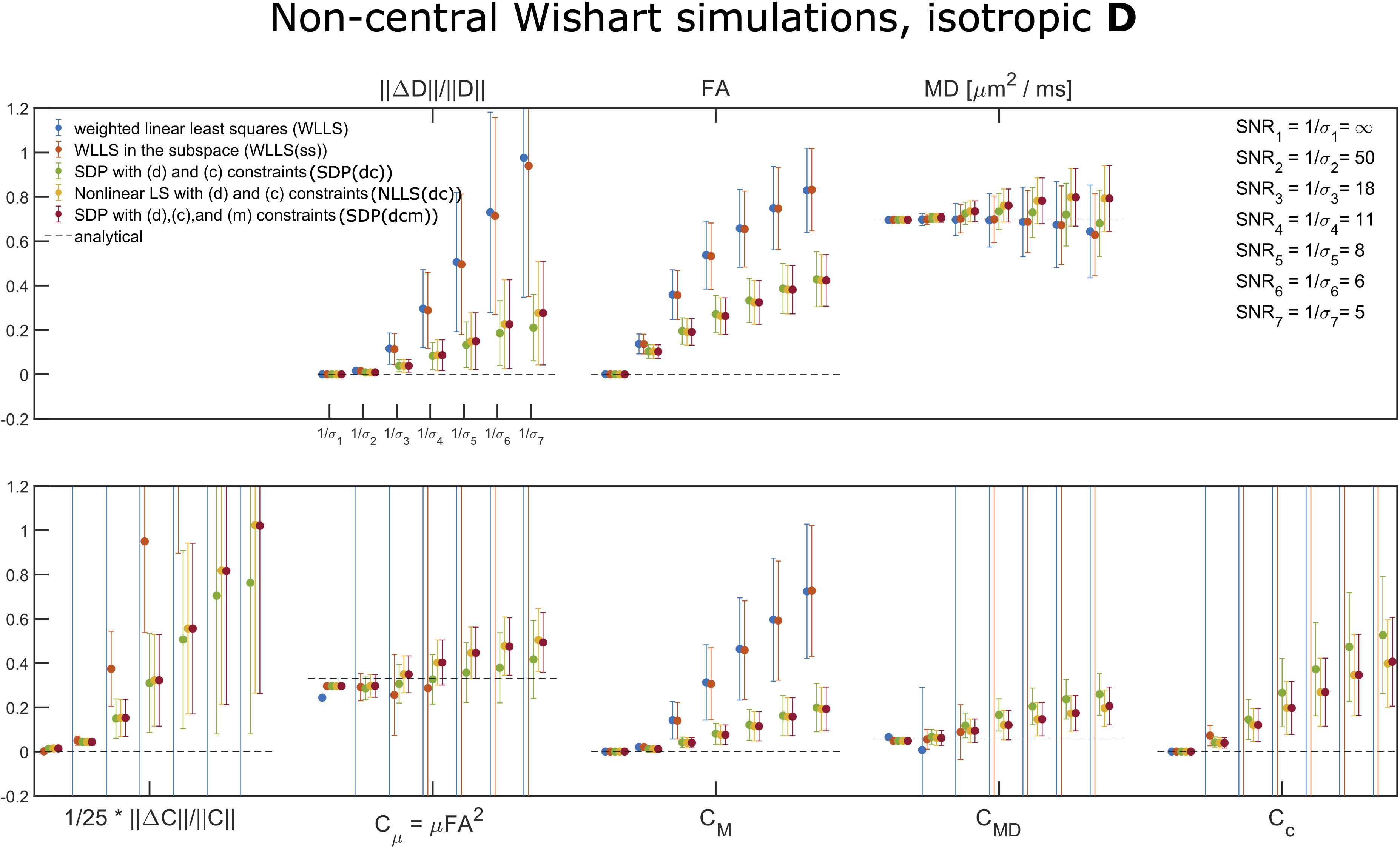
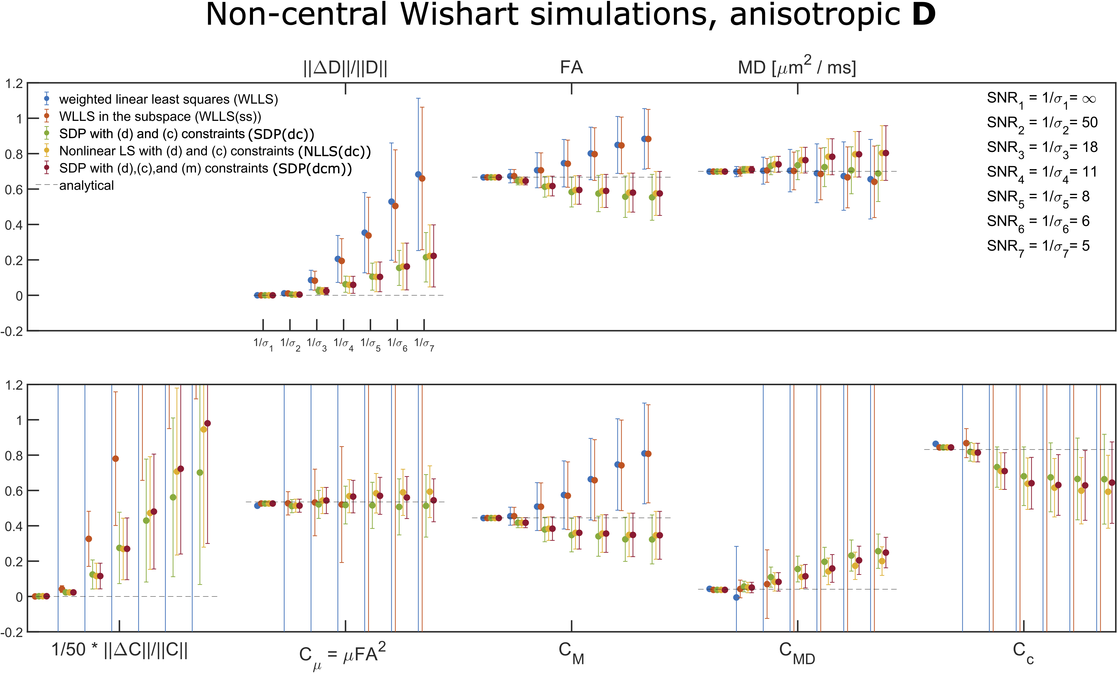
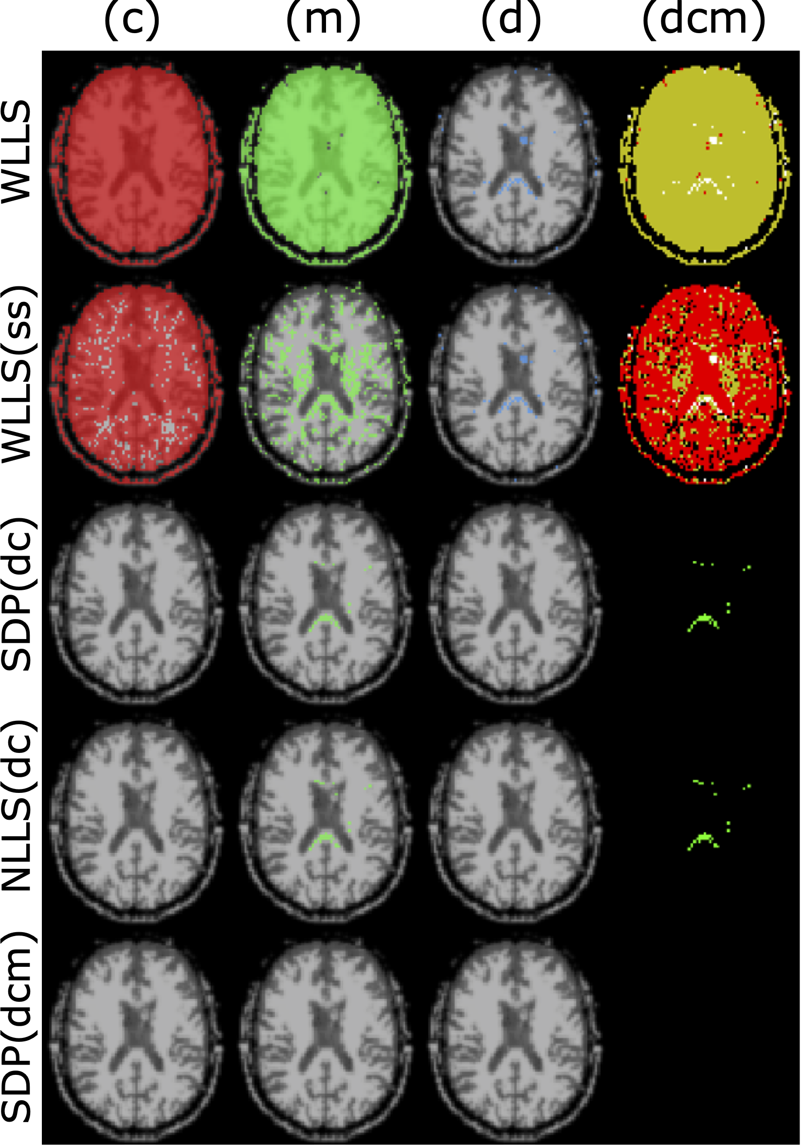
Figures 2 and 3 show the results of the simulations performed on the 81-measurement protocol, modeling isotropic and anisotropic $$$\hat D_{ij}$$$, respectively. Generally, applying the positivity constraints vastly improves robustness to noise.Figure 4 shows where conditions (d), (c), and (m) are violated for the unconstrained fits (first two rows), and constrained fits (last three rows). Condition (c) is violated almost everywhere if constraints are not applied.
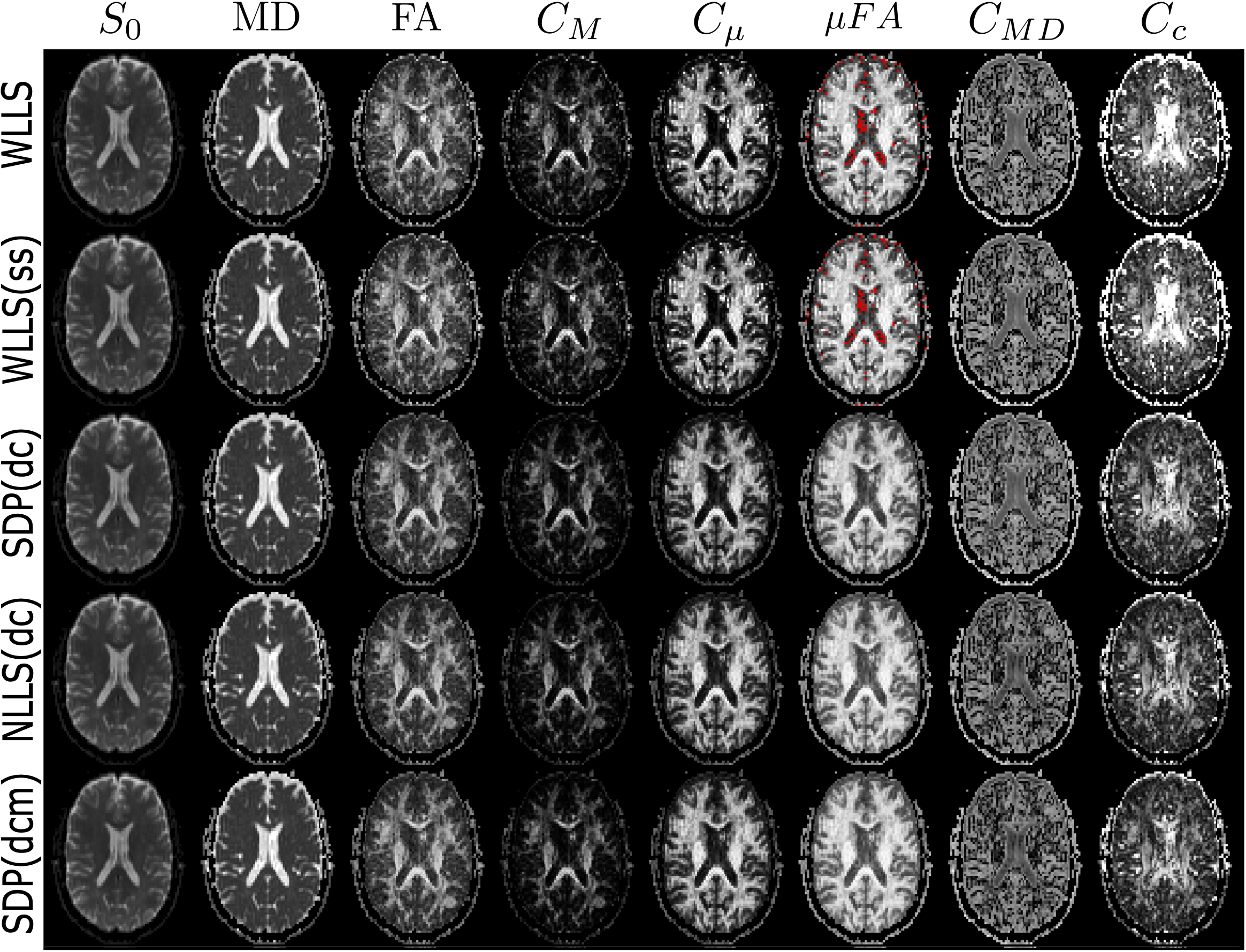
Figure 5 contains the scalar maps obtained from the QTI analysis when employing unconstrained fitting routines and our QTI+ framework. Interestingly, the invariants obtained with the developed framework exhibit a generally smoother appearance even though the analysis is performed on a voxel-by-voxel basis. This suggests higher noise resilience when constraints are enforced during the fitting.
Discussion
We considered imposing three constraints on the estimated mean and covariance tensors although, each and every diffusion tensor in the underlying DTD has to be positive-semidefinite. However, imposing such a strong condition without attempting to solve an extremely ill-posed problem that involves the reconstruction of the actual DTD3,13,16 is likely to be infeasible in noisy conditions. Interestingly, non-negativity of each microscopic diffusion tensor implied the (m) condition, which seemed to have a minor effect in our analyses. Much of the improvement is already obtained through imposing the (d) and (c) conditions, suggesting that the SDP(dc) routine can be employed with relative confidence, which makes the overall estimation computationally inexpensive compared to the full framework.Conclusion
We presented QTI+, a new estimation framework for QTI that respects three positivity conditions arising from the nature of the quantities estimated. We demonstrated that this leads to signi ficant improvements in the accuracy of the estimates.Acknowledgements
This project was financially supported by the Swedish Foundation for Strategic Research (AM13-0090 and Multimodal Guidance in Neurosurgery), the Swedish Research Council 2016-04482, Linköping University (LiU) Center for Industrial Information Technology (CENIIT), LiU Cancer, VINNOVA/ITEA3 17021 IMPACT, and Analytic Imaging Diagnostic Arena (AIDA).
Tom Dela Haije and Aasa Feragen were supported by the Center for Stochastic Geometry and Advanced Bioimaging and by a block stipendium, both funded by the Villum Foundation (Denmark).
References
1.
Cory, D.G., Garroway, A.N., Miller, J.B.
Applications of spin transport as a probe of local geometry. Polym Preprints
1990;31:149.
2. Westin, C.F., Knutsson, H., Pasternak, O., Szczepankiewicz, F., Özarslan, E., van Westen, D., Mattisson, C., Bogren, M., O'Donnell, L.J., Kubicki, M., Topgaard, D., Nilsson, M.. Q-space trajectory imaging for multidimensional diffusion MRI of the human brain. NeuroImage 2016;135:345-362.
3. Jian, B., Vemuri, B.C., Özarslan, E., Carney, P.R., Mareci, T.H. A novel tensor distribution model for the diffusion-weighted MR signal. NeuroImage 2007;37(1):164-176.
4.
Basser, P.J.,
Mattiello, J., LeBihan, D. Estimation of the effective self-diffusion tensor from the NMR spin
echo. J Magn Reson B 1994a;103(3):247-254.
5. Özarslan E., Shemesh N., Koay C.G., Cohen Y., Basser P.J. Nuclear magnetic resonance characterization of general compartment size distributions. New J Phys 2011; 13:015010.
6. https://github.com/markus-nilsson/md-dmri
7. Dela Haije, T., Özarslan, E., Feragen, A. Enforcing necessary nonnegativity constraints for common diffusion MRI models using sum of squares programming. NeuroImage 2020;209:116405.
8. Liu, C., Bammer, R., Acar, B., Moseley, M.E. Characterizing non-Gaussian diffusion by using generalized diffusion tensors. Magn Reson Med 2004;51(5):924–937.
9. Jensen, J.H., Helpern, J.A., Ramani, A., Lu, H., Kaczynski, K. Diffusional kurtosis imaging: the quantification of non-Gaussian water diffusion by means of magnetic resonance imaging. Magn Reson Med 2005;53:1432–1440.
10. Tournier, J.D., Calamante, F., Connelly, A. Robust determination of the fibre orientation distribution in diffusion MRI: Non-negativity constrained super-resolved spherical deconvolution. NeuroImage 2007;35(4):1459–1472.
11. Özarslan E., Koay C.G., Shepherd T.M., Komlosh M.E., Irfanoglu M.O., Pierpaoli C., Basser P.J. Mean apparent propagator (MAP) MRI: a novel diffusion imaging method for mapping tissue microstructure. NeuroImage, 2013; 78:16–32.
12. Mayerhofer, E. On the existence of non-central Wishart distributions. J Multivariate Anal 2013;114:448-456.
13. Shakya, S., Batool, N., Özarslan, E., Knutsson, H. Multi-fiber reconstruction using probabilistic mixture models for diffusion MRI examinations of the brain. In: Schultz, T., Özarslan, E., Hotz, I., editors. Modeling, Analysis, and Visualization of Anisotropy, Cham: Springer International Publishing, p. 283-308, 2017.
14. https://github.com/filip-szczepankiewicz/fwf_seq_resources/tree/master/GE
15. Szczepankiewicz
F, Hoge S, Westin CF. Linear, planar and spherical tensor-valued diffusion MRI
data by free waveform encoding in healthy brain, water, oil and liquid
crystals. Data Brief. 2019;25:104208.
16. Najmudeen M.K., Gasbarra D., Basser P.J. A theoretical framework for representing and estimating a normal diffusion tensor distribution. In: Proc Intl Soc Mag Reson Med. volume 28; 2020.
Figures