Introduction

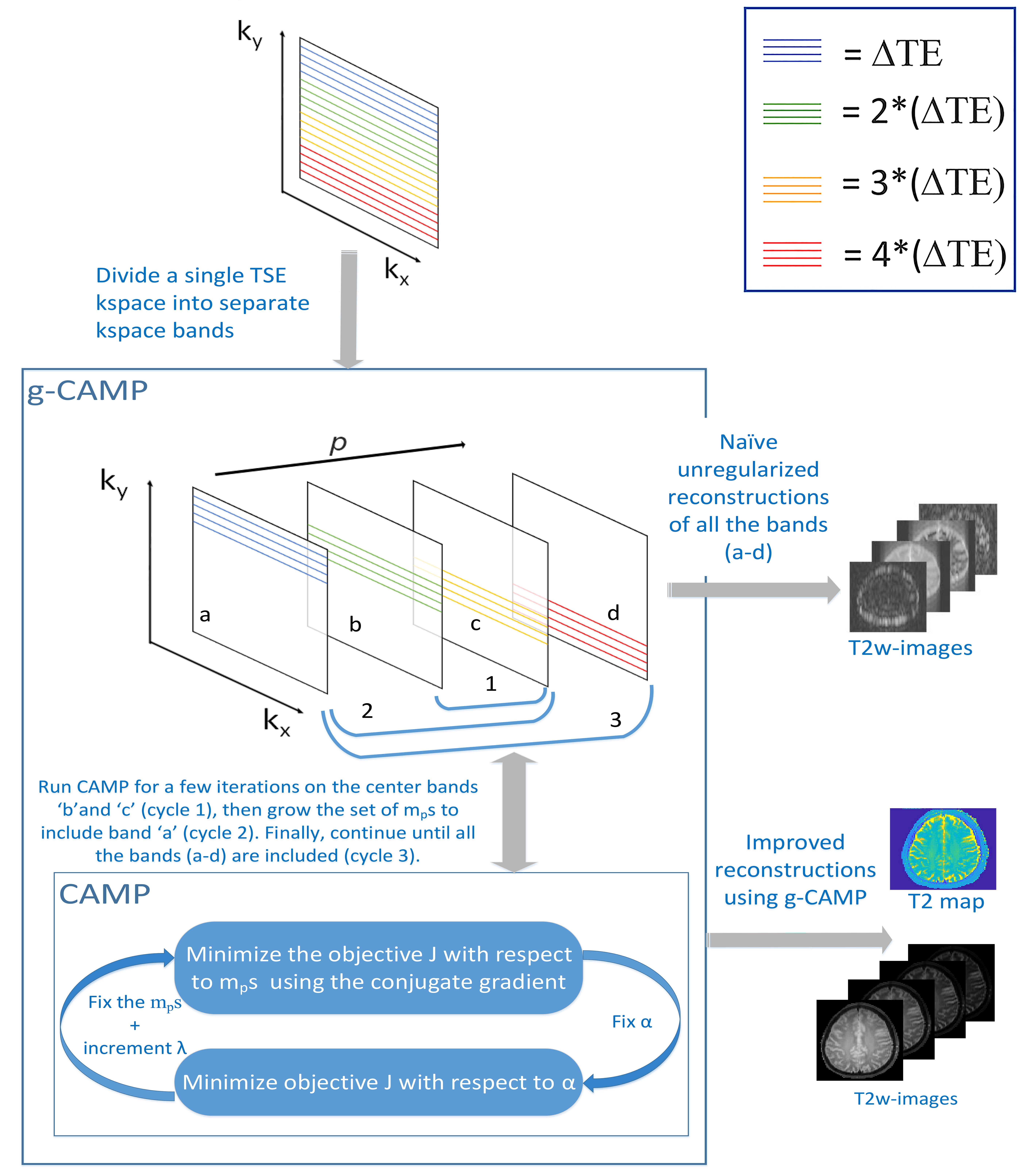
Quantitative T2-maps have many advantages over grayscale T2w-images as they show greater consistency across multi-site studies and for machine learning applications ¹, but their long acquisition time makes them difficult to perform routinely. While many groups have shown that faster T2-mapping can be accomplished by appropriate regularization across the echo series, prior work has focused on evenly spaced sampling at each echo. ² However, a standard T2w-scan can be regarded as a kind of undersampled T2-mapping sequence with block-like k-space sampling at each echo. Because CAMP ³ (Constrained Alternating Minimization for Parameter mapping) is a very general reconstruction scheme compatible with any acquisition pattern across the echoes, the CAMP extension to g-CAMP (growing CAMP) was found to generate quantitative T2-maps from data traditionally acquired for a single grayscale T2w-image. CAMP alternates between optimizing the image series and the parameter map, but it does so by minimizing a single cost-function that incorporates both (1) consistency between each individual parameter image and its k-space data and (2) adherence of the image series to the relaxometry model for each pixel. In g-CAMP, the standard CAMP method ³ is applied first to the center two bands of k-space, then it grows in each direction until it includes all the bands of k-space from the whole T2w-dataset.

Methods

CAMP
In MR parameter mapping, the complete MRI signal vector $$$S(k)$$$ is regarded as a series of signal vectors $$$S_p (k)$$$, each of which samples the k-space $$$k$$$ of a complex weighted image $$$m_p$$$ acquired at different parameter encoding values (e.g., echo time TE), through the encoding matrix $$$E_p$$$ for a total of $$$p$$$ images, where $$$p$$$ is also the number of echo times sampled.
As described in ³, the relationship of each parameter map relative to the previous one is $$$m_{(p+1)} (x)=m_p (x)α(x),$$$ where $$$α(x)=exp(\frac{-p∆TE}{T_2 (x)})$$$. Incorporating this, the CAMP objective function is $$$J=J_1+J_2+J_3$$$, where $$$J_1=∑_{(p=1)}^P‖S_p-E_p m_p ‖^2$$$ is the data fidelity term, $$$J_2=τ∑_{(p=1)}^PTV(m_p )$$$ is a TV-norm regularization term, and finally, $$$ J_3=λ∑_{(x=1)}^N∑_{(p=1)}^{(P-1)}‖m_{(p+1)} (x)-α(x) m_p (x)‖^2 $$$ is the CAMP constraint. $$$τ$$$ and $$$λ$$$ are both weighting parameters. The CAMP objective function $$$J$$$ is alternately minimized with respect to $$$m_p$$$ (fixed $$$α$$$) using a non-linear conjugate-gradient method (Polak-Ribiere). ⁴ It is then minimized with respect to $$$α$$$ (fixed $$$m_p$$$), keeping in mind that $$$α$$$ is real. This loop is repeated until both $$$m_p$$$ and $$$α$$$ converge.

g-CAMP
As shown in Figure 1, the g-CAMP algorithm starts by using only the two center bands of k-space. A CAMP reconstruction on these two bands continues for several iterations until it converges. Except for the middle two images, each image is initialized before entering the CAMP loop as a uniformly scaled version of the previously reconstructed neighboring image, using a scale factor derived from the middle bands of data. In addition, the phase of each $$$m_p$$$ is assumed to be that of the standard grayscale T2w-image. This is implemented by incorporating that phase into $$$E_p$$$ and forcing each update to the $$$m_p$$$ series to be real.

Simulation
Data were simulated to mimic a single T2w-acquisition, where k-space is acquired blockwise across 8 echoes, and the center of k-space was acquired at the 4th echo. Digital-phantoms for each echo time were generated using a T2-template and a proton-density (PD) template, and appropriate gradient and coil encodings were applied to each phantom to generate the multi-echo data. Coil weightings were derived from experimental coil profiles in an eight-channel coil. Random Gaussian noise with zero mean and a standard deviation of 2% of the ℓ2-norm of the signal was added to the data.

Imaging
T2w-images were acquired on a 3T MRI scanner (MAGNETOM Trio Tim, Siemens Healthcare, Erlangen, Germany). A Cartesian TSE sequence was used with TR=2500 ms, ETL= 8 and TE=21 ms, with a base-resolution of 128, 3mm slice thickness.

Results

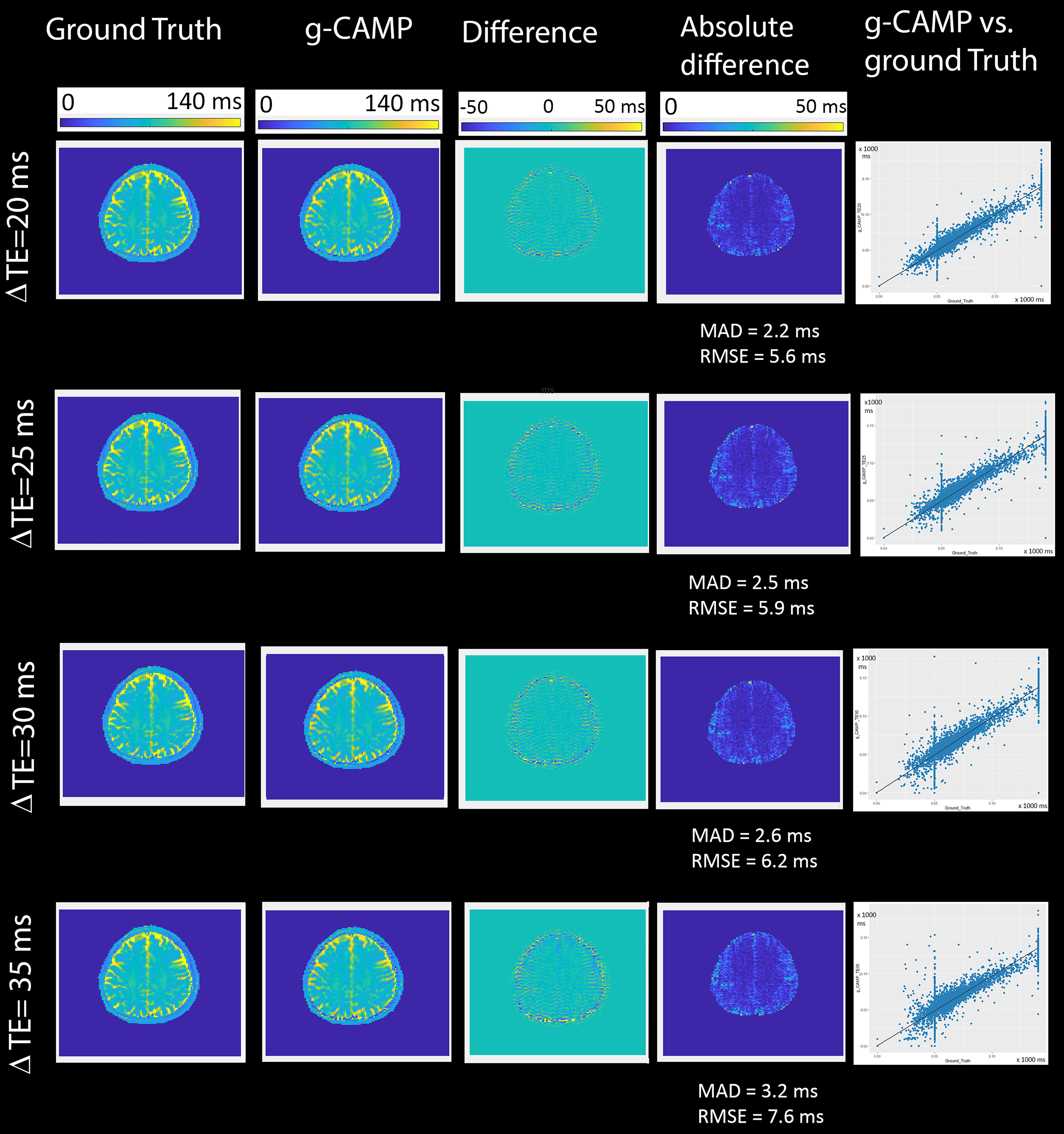
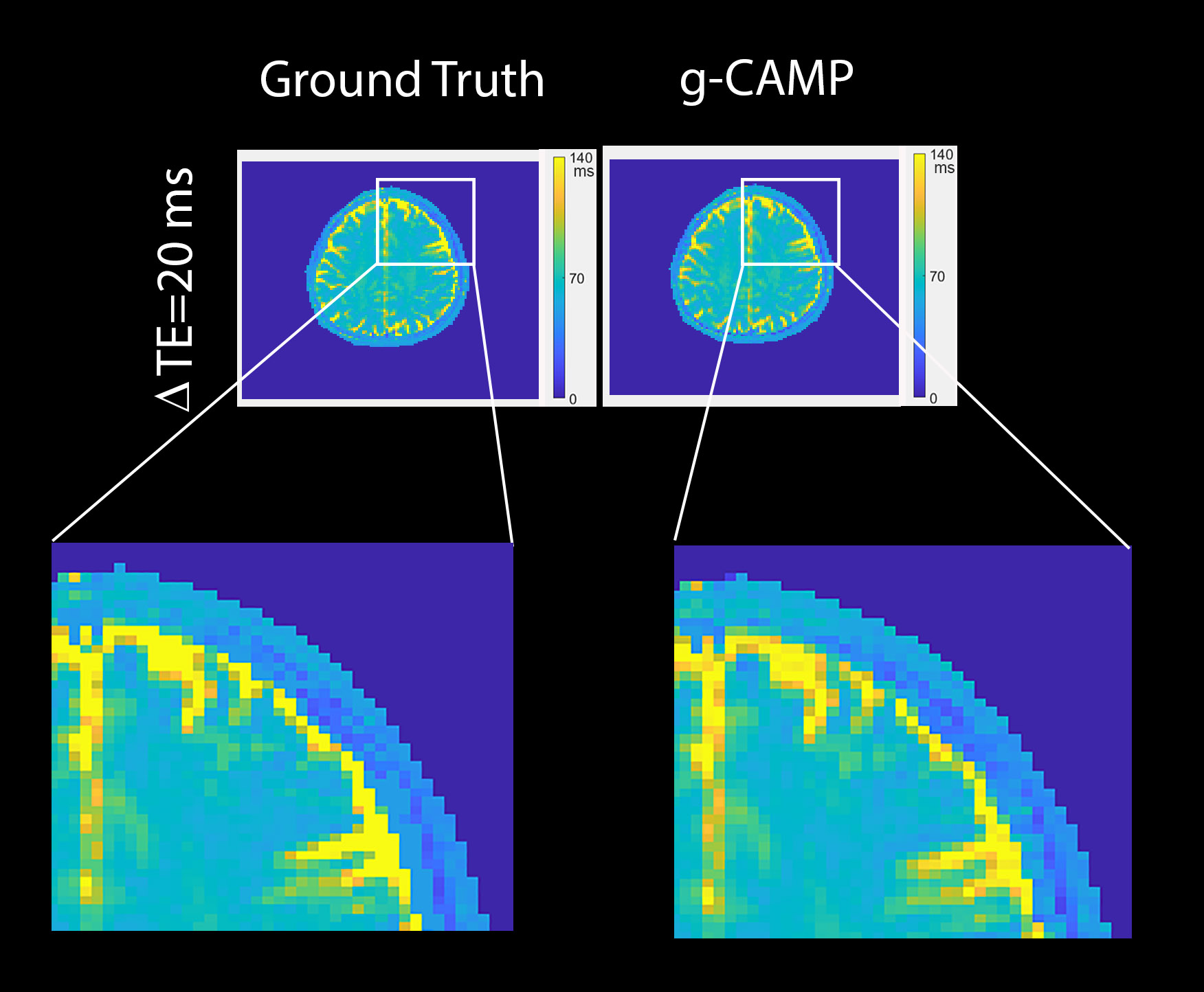
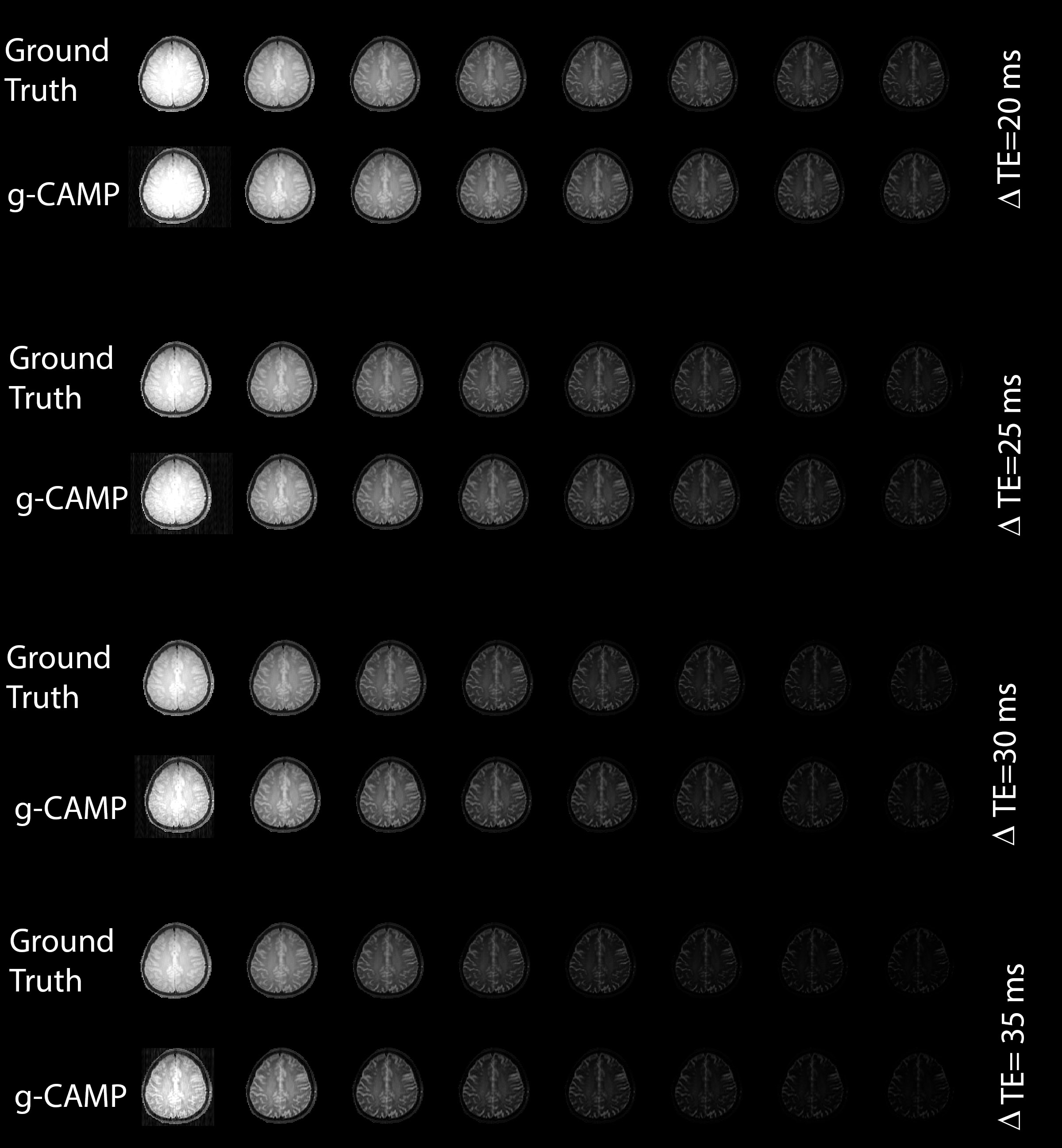
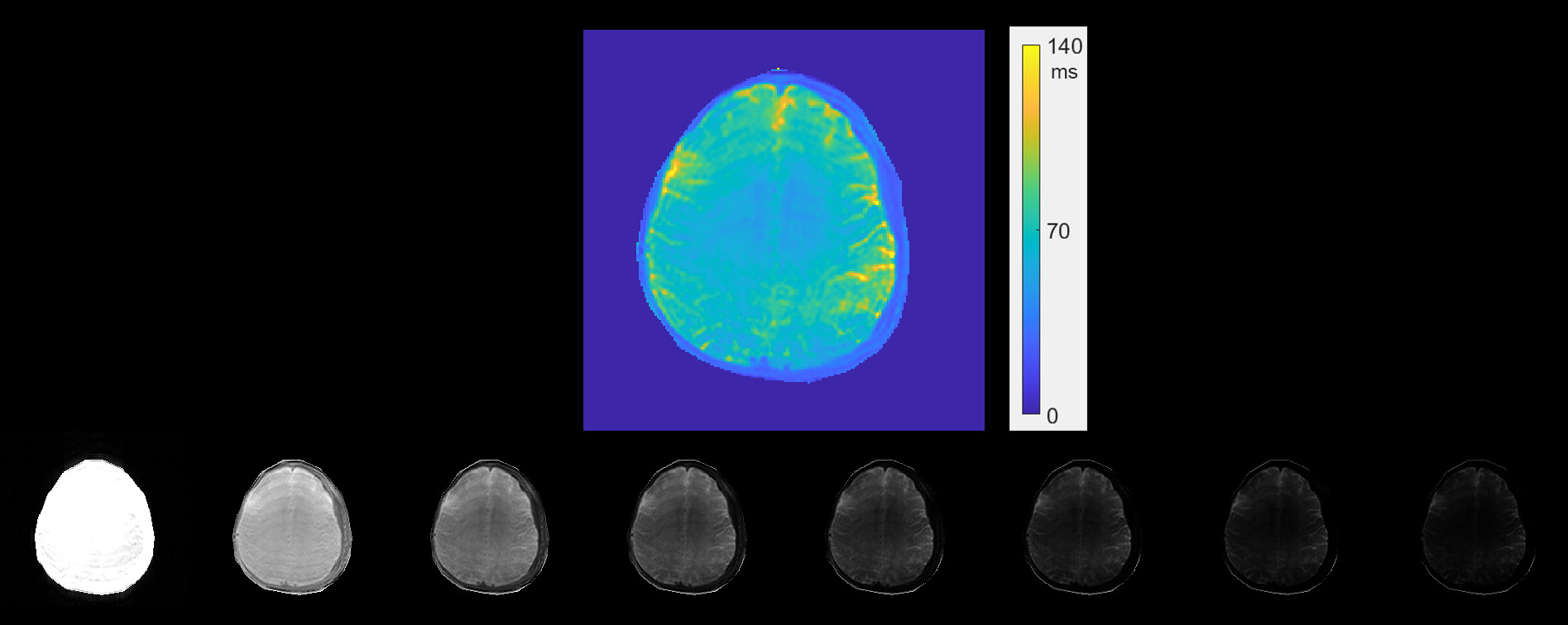
The Cartesian simulation results in Figure 2 demonstrate g-CAMP applied to different echo spacings, where the difference images between ground truth and g-CAMP reconstructions show median absolute deviation (MAD) errors between 2.2 to 3.2 ms and root-mean-square-error (RMSE) between 5.6 to 7.6 ms. A scatter plot of ground truth vs. reconstructed T2 values produces an adjusted R² of 0.9606-0.9865. A zoomed-in box of the ΔTE=20 ms T2-map (Figure 3) shows that the resolution is not compromised by g-CAMP. Figure 4 shows the full image series generated from each reconstruction which, like the T2-maps, is in good agreement with the ground truth. Having done extensive simulations, we are now in the process of applying g-CAMP to experimental data. Even the application of the previous simpler algorithm (CAMP) to existing T2w data shows promise (Figure 5), with contrast and numerical values consistent with the literature.

Discussion and Conclusion

This work demonstrates the potential of g-CAMP to retrospectively reconstruct quantitative T2-maps from data acquired for a standard single-contrast T2w-acquisition. While this work applies g-CAMP to quantitative T2-mapping, g-CAMP can also be extended to T1 relaxation by adding an intercept to the relaxation model. Therefore, there may be potential to retrospectively process TSE and MPRAGE imaging data to calculate accurate T2 and T1-maps respectively.

Acknowledgements

We note that both Dr. Galiana and Dr. Tagare contributed equally as senior authors on this work. This work was funded by the National Institutes of Health under R01EB022030, R01EB012289, 4R01 EB016978, and K01EB16897.