Introduction

Balanced steady state free precession (bSSFP) imaging is an SNR-efficient modality with high fluid-tissue contrast. These properties ensure its diagnostic capacity for imaging in regions such as cardiac and the internal auditory canal (IAC)¹. bSSFP would be even more valuable clinically if it provided quantitative tissue and environment parameter maps². Previously, a geometric solution (GS)³ based on the elliptic signal model (ESM) using 4 phase-cycled bSSFP images demonstrated the capacity to generate artifact-free images with an off-resonance field map^4,5. When coupled with complementary ESM computations such as the algebraic solution (AS)⁶, it is apparent that quantitative MR parameters may be realized analytically using the bSSFP ESM. While numerical methods such as the PLANET⁷ and DESPOT2⁸ exist, exact bSSFP parametric maps have yet to be calculated. Here the first analytical computation of $$$T_2$$$ relaxation and source ESM parameters using bSSFP is formulated via an exact geometric methodology.

Theory

Eq.(1) describes the ESM. $$$\theta=\Delta\omega\cdot{TR}+\psi$$$ is the off-resonant phase accumulation per repetition time $$$TR$$$ for precession frequency off-resonance $$$\Delta\omega$$$, $$$\varphi=-\Delta\omega\cdot{TE}$$$ represents the phase accumulation at echo time $$$t=TE$$$ and $$$\psi$$$ is the phase cycling increment.
$$I(\theta,\psi)=M\frac{1-ae^{i(\theta+\psi)}}{b\,\mathrm{cos}(\theta+\psi)}e^{i\varphi}\tag{1}$$
Eq.(2) defines the ESM parameters $$$|M|,a,b$$$, in terms of the equilibrium magnetization $$$M_0$$$, flip angle $$$\alpha$$$, $$$TR$$$, and relaxation times $$$T_1$$$ and $$$T_2$$$.
$$\begin{aligned}E_1&=\mathrm{exp}(-TR/T_1)\\a&=E_2=\mathrm{exp}(-TR/T_2)\\|M|&=\frac{M_0(1-E_1)\,\mathrm{sin}\alpha}{1-E_1\,\mathrm{cos}\alpha-E_2^2(E_1-\mathrm{cos}\alpha)}\\b&=\frac{E_2(1-E_1)(1+\mathrm{cos}\alpha)}{1-E_1\,\mathrm{cos}\alpha-E_2^2(E_1-\mathrm{cos}\alpha)}\end{aligned}\tag{2}$$
Four unique datasets are formed at phase cycling increments $$$\psi_1=0^{\circ},\psi_2=90^{\circ},\psi_3=180^{\circ},\psi_4=270^{\circ}$$$ respectively.
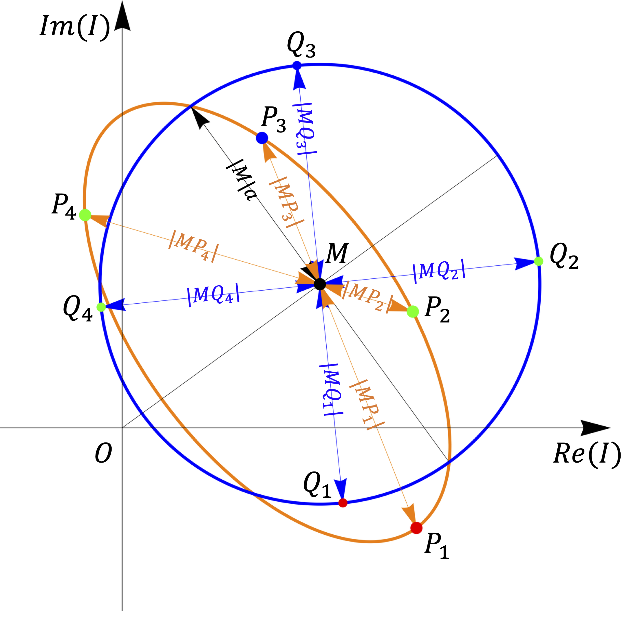
As shown by the orange signal ellipse curve in Fig. 1, point $$$P_i$$$ represents the signal $$$I_i$$$ with the phase cycling increment $$$\psi_i$$$. The blue circle with center at $$$M$$$ obtained by transforming points $$$P_i$$$ on the signal ellipse to points $$$Q_i$$$ is define by $$$J(\theta,\psi)$$$:
$$J(\theta,\psi)=I(\theta,\psi)(1-b\,\mathrm{cos}(\theta+\psi))=|M|e^{i\varphi}(1-ae^{i\theta})\tag{3}$$
The geometric cross-point $$$M=(M_x,M_y)$$$ is calculated via the geometric solution as described by Xiang and Hoff³.
The ratio of the distances $$$|MP_i|$$$ from signal points $$$P_i$$$ to the cross-point $$$M$$$ permits a geometric calculation of $$$b$$$ (and $$$\theta$$$):
$$b\,\mathrm{cos}\theta=\frac{|MP_1|-|MP_3|}{|MP_1|+|MP_3|},b\,\mathrm{sin}\theta=\frac{|MP_4|-|MP_2|}{|MP_2|+|MP_4|}\\b=\sqrt{\left(\frac{|MP_1|-|MP_3|}{|MP_1|+|MP_3|}\right)^2+\left(\frac{|MP_4|-|MP_2|}{|MP_2|+|MP_4|}\right)^2}\tag{4}$$
Coordinates $$$Q_i$$$ may then be computed by multiplying the signal coordinates of point $$$P_i$$$ by $$$(1\pm{b}\,\mathrm{cos}\theta)$$$ or $$$(1\pm{b}\,\mathrm{sin}\theta)$$$ from Eq.(4). The intersection of the circle and ellipse indicates that the circle $$$J$$$ radius $$$|MQ_i|=|M|a$$$. Therefore, $$$a$$$ may be computed once for each of the four transformed phase-cycled points $$$Q_i$$$:
$$\begin{aligned}a_i&=|MQ_i|/|M|\\\overline{a_{rms}}&=\sqrt{(a_1^2+a_2^2+a_3^2+a_4^2)/4}\end{aligned}\tag{5}$$
An $$$a$$$ map can be obtained by calculating the root mean square of $$$a_i$$$, and a $$$T_2$$$ map using Eq.(2) $$$a=\mathrm{exp}(-TR/T_2)$$$.

Methods

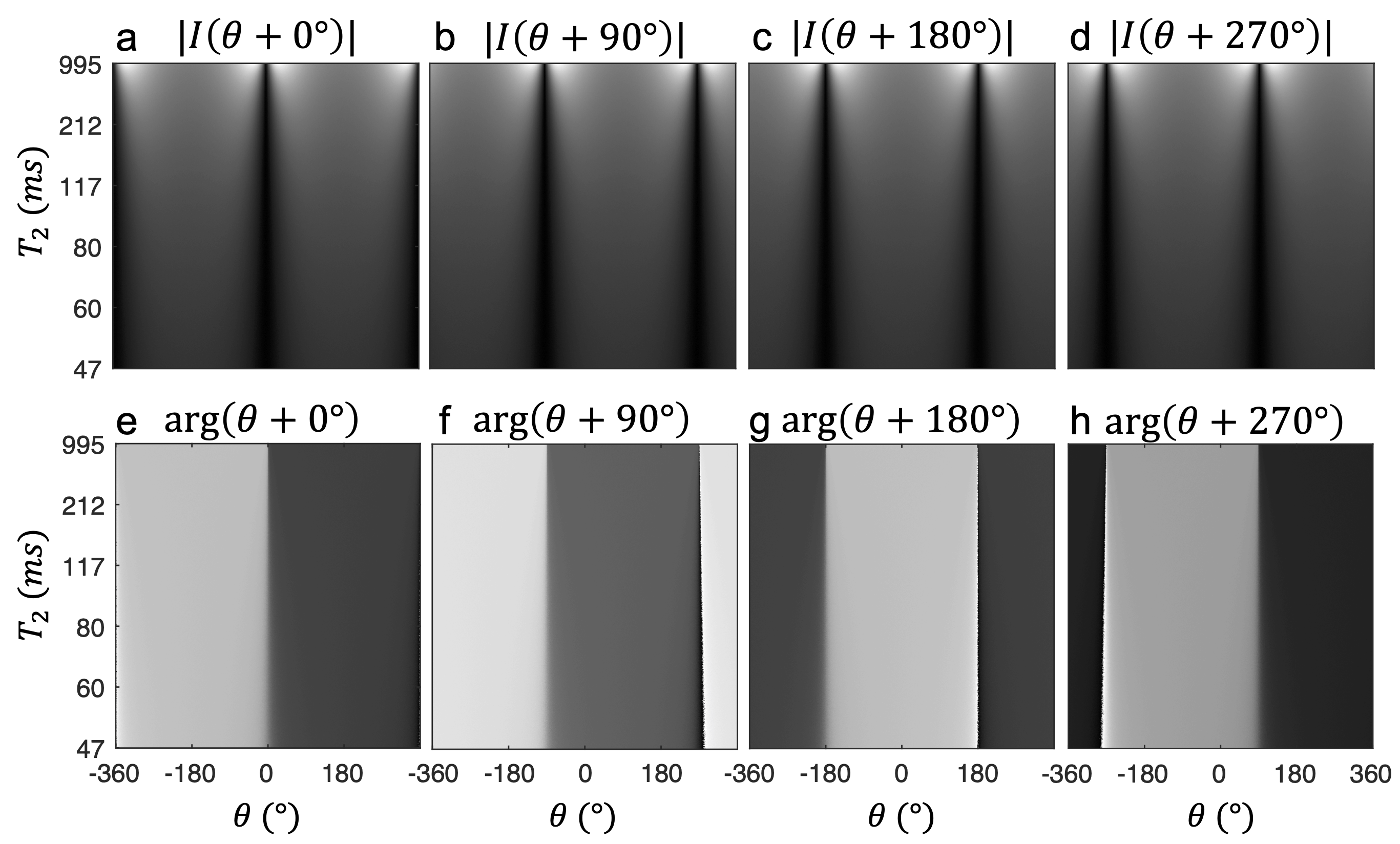
Four phase-cycled images are simulated using phase cycling increments $$$\psi=0^{\circ},90^{\circ},180^{\circ}\,\text{and}\,270^{\circ}$$$, flip angle $$$\alpha=30^{\circ}$$$ and $$$TR=10ms$$$. $$$T_1$$$ is held constant at $$$1000ms$$$. $$$T_2$$$ is varied from $$$47ms$$$ to $$$995ms$$$ such that $$$a$$$ varies from $$$0.81$$$ to $$$0.99$$$ and $$$b$$$ varies from $$$0.25$$$ to $$$0.87$$$ vertically. The off-resonant angle $$$\theta$$$ varies from $$$-2\pi$$$ to $$$2\pi$$$ horizontally. Bivariate gaussian noise set to $$$2\%$$$ of the mean intensity is also added.
The solution for $$$a,b$$$ and $$$T_2$$$ was computed pixel-by-pixel with signal real parts $$$x_i$$$, imaginary parts $$$y_i$$$ and the geometric solution cross-point $$$M=(M_x,M_y)$$$. The Total Relative Error (TRE) of each analytical solution $$$f_i(x,y)=a,b\,\text{and}\,\theta$$$ over all pixel values $$$x,y$$$ is computed by
$$TRE(f)=\frac{\sqrt{\sum_{x,y}[f_i(x,y)-f_g(x,y)]^2}}{\sum_{x,y}f_g(x,y)}\tag{6}$$
with respect to the gold standard $$$f_g$$$. Extended-size datasets were employed to permit computation of TRE vs. $$$a,T_2$$$ and $$$\theta$$$. $$$11$$$ datasets of similar simulated images were generated with Gaussian noise percentage ranging from $$$0\%$$$ to $$$10\%$$$ for the TRE vs. noise computation.

Results

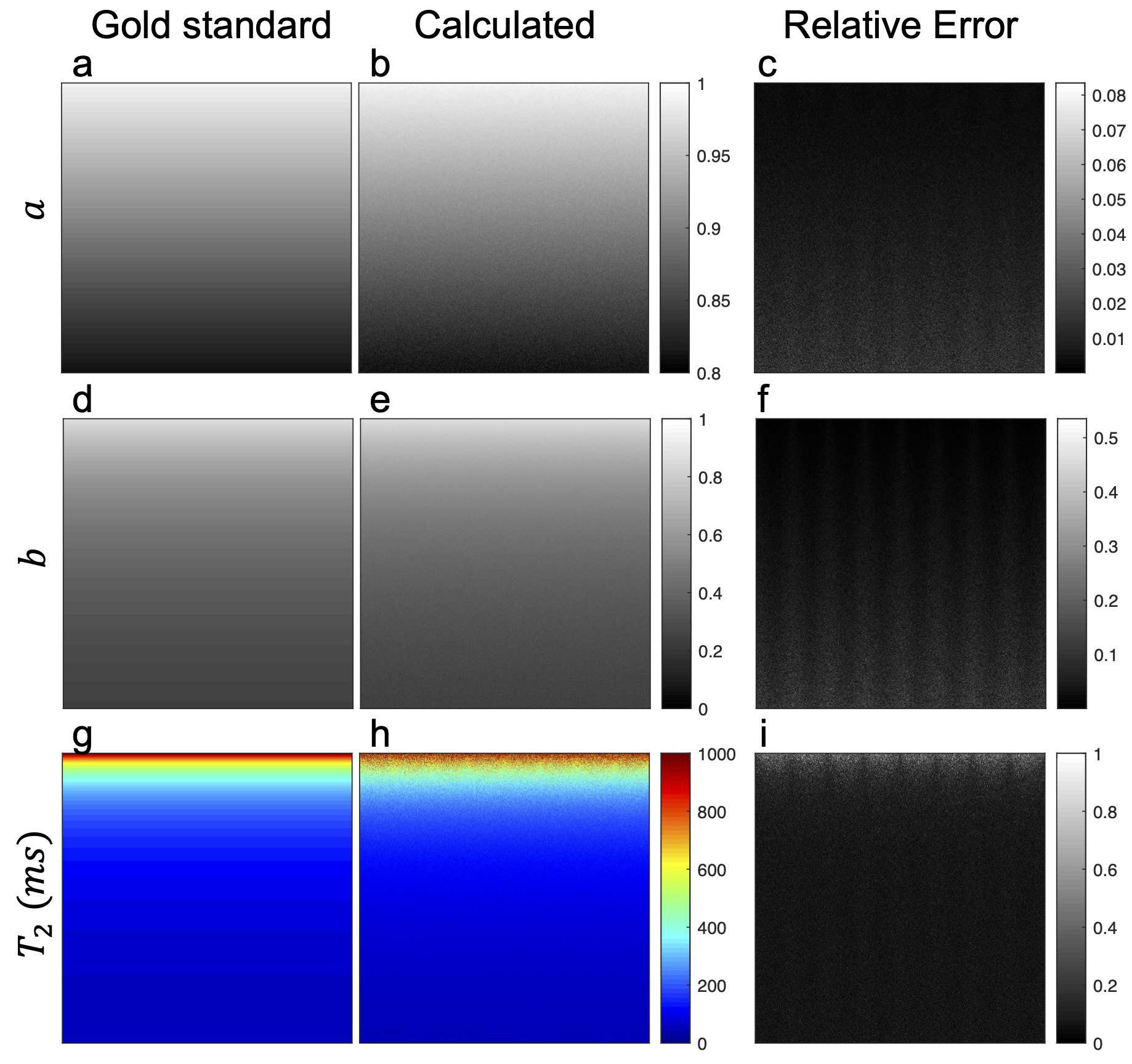
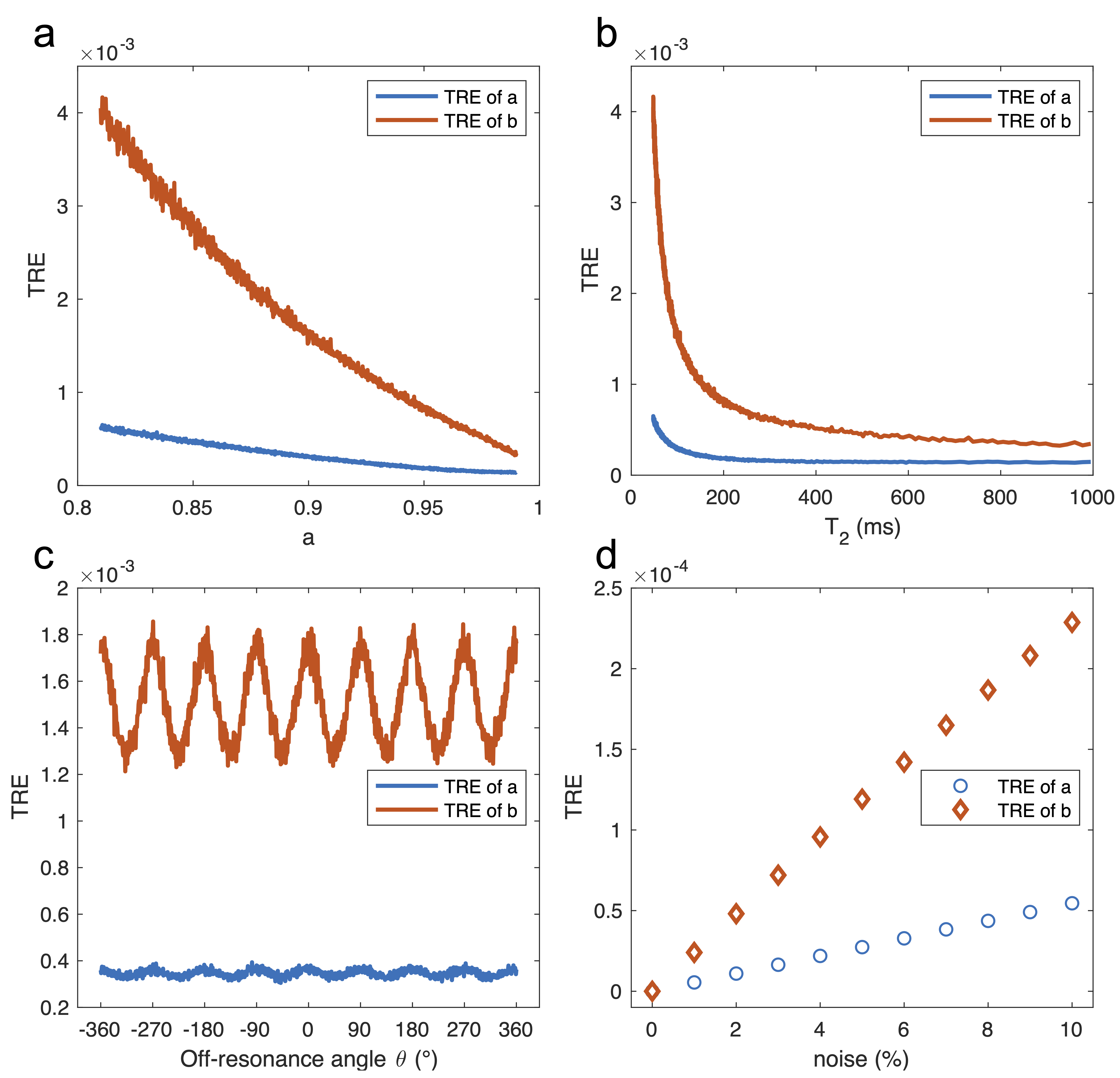
Fig.3 shows good correspondence between the $$$a,b$$$ and $$$T_2$$$ gold standard and calculated analytical solution maps. Relative error is calculated and shown in the right column, indicating accurate contrast with some increased $$$\theta$$$-dependent variance.
Fig.4a and Fig.4b depict the TRE of $$$a$$$ and $$$b$$$ parameters calculated with varying $$$T_2$$$, and are plotted respectively against $$$T_2$$$ itself and the $$$a(T_2)$$$ value. TRE of the solutions gradually decrease as $$$T_2$$$ value increases.
Fig.4c shows a periodic dependency of the $$$a$$$ and $$$b$$$ TRE on off-resonant angle $$$\theta$$$. Fig.4d shows increased TRE as added noise increases.

Discussion

A 4-point geometric solution to $$$a,b\,\text{and}\,T_2$$$ is formulated, which realizes the first analytical computation of the relaxation parameter $$$T_2$$$ using the ESM of bSSFP. The solution to $$$a,b\,\text{and}\,T_2$$$ is exact and without error in noiseless scenarios. With noise present, the $$$a$$$ solution demonstrates relatively little error, whereas the calculated $$$b$$$ shows a stronger periodic variation from the gold standard at $$$\theta=N\pi/2$$$. The ESM indicates that when $$$b\mathrm{cos}\theta$$$ or $$$b\mathrm{sin}\theta$$$ approach zero at $$$N\pi/2$$$, added noise may relatively dominate signal terms. This is exacerbated by squaring the terms in the calculation of $$$b$$$. Note that it is the $$$b$$$-solution variance (and not contrast/level) that depends on $$$\theta$$$, and that the slight $$$\theta$$$-dependence of the GS solution variance⁶ may also contribute.
The calculated $$$T_2$$$ map is accurate when $$$T_2$$$ is small ($$$<200ms$$$). But the inverse logarithm computation $$$a=\mathrm{exp}(-TR/T_2)$$$ causes instability when $$$a$$$ is close to 1. Optimized processing of the averaged $$$a$$$ value should improve $$$T_2$$$ map accuracy.

Conclusion

The first analytic solution for $$$T_2$$$ using the ESM of bSSFP is shown to be relatively robust for calculations of ESM parameters $$$a$$$ and $$$b$$$ under variation of noise levels, $$$T_2$$$ values and band proximity. This inspires clinical application of this novel GS-scaled method to add bSSFP parametric maps to artifact-free images.

Acknowledgements

No acknowledgement found.