2603

Extracting information from diffusion MRI models to visualize the adequacy of acquisition protocols

Samuel St-Jean^1,2, Filip Szczepankiewicz², Christian Beaulieu¹, and Markus Nilsson²
¹University of Alberta, Edmonton, AB, Canada, ²Clinical Sciences Lund, Lund University, Lund, Sweden

Synopsis

Parameter degeneracies and numerical fitting issues are the bane of diffusion MRI modelling. In this work, we present a framework using convex optimization to fit diffusion MRI models efficiently similarly to magnetic resonance fingerprinting. We also show how the singular value decomposition of these models can help to visualize how well the parameter space of a given model is sampled by a given acquisition protocol. Results on b-tensor encoded datasets and datasets leveraging multiple echo times literally show how these additional measurement dimensions disentangle model parameters better compared to traditional sequences.

Introduction

Diffusion MRI allows non-invasive investigation of tissue microstructure, but the optimal acquisition scheme for a given model is not known. Additionally, there are numerical challenges associated with fitting nonlinear equations such as parameter degeneracies and long processing times¹. In this work, we propose a framework which uses a series of inner products of the signal for fitting, similar to magnetic resonance fingerprinting (MRF)², where small convex problems are solved instead of one big least-square problem. We also show how singular value decomposition (SVD) can be used to visualize the parts of the model contributing most to the data, allowing a ranking of different protocols and how well they respond to a given model before acquiring data.

Theory

The central property of this work is the linearity of the inner product and its invariance to multiplication by an orthogonal matrix. For a two-compartment model, the contribution of each compartment can be separated from the signal fractions as show by Equation 1 such that
$$\frac{<S,f_1C_1+f_2C_2>}{||S|| ||f_1C_1+f_2C_2||}=\frac{f_1<S,C_1>+f_2<S,C_2>}{||S||\sqrt{f_1^2||C_1||^2+f_2^2||C_2||^2+2f_1f_2<C_1,C_2>}}$$
With <,> the inner product, ||,|| the associated norm and $$$C_i$$$ the signal for compartment $$$i$$$ and $$$f_i$$$ the signal fraction. A discrete database of signals is constructed with Equation 1, the acquisition parameters, and a grid of model parameters. The highest value of the inner product gives the best matching parameters for the signal. The SVD is used to project the model to a smaller parameter space which captures the important information. Analysing the eigenvalues of the model for a given acquisition shows how well it captures the model features.

Datasets

Four previously published datasets^3,4 were powder-averaged and used for this study. Two were preprocessed datasets from the Human Connectome Projects (HCP)^5,6 with b-values of [0,1000,2000,3000] and [0,1000,3000,5000,10000] s/mm². One was acquired using b-tensor encoding with b_delta = [0.63,1] and b-values of [100,1000,2000,2500,5000] s/mm². The last dataset was acquired with the same b-values, b_delta = [0.6,1] and TE = [63,85,130] ms and corrected for eddy current and motion as described previously⁷.

Methods

A two compartment stick-and-zeppelin model purportedly capturing intra- and extra-axonal diffusion^2,3 was used for the HCP datasets as defined by
$$C_1=\sqrt{\pi/4}\text{erf}(\sqrt{bD_{\text{par}}})/\sqrt{bD_{\text{par}}}$$
and
$$C_2=\sqrt{\pi/4}\exp{(-bD_{\text{par}}})\text{erf}(\sqrt{b(D_{\text{par}}-D_{\text{perp}}})/\sqrt{b(D_{\text{par}}-D_{\text{perp}})}$$
where b is the encoding strength, D_par and D_perp the diffusivities, and erf is the error function. For the case of b-tensor encoding, $$$C_1$$$ and $$$C_2$$$ become
$$C_1=\exp{(-bD(1-b_{\text{delta}})})\sqrt{\pi/(4x)}\text{erf}(\sqrt{x})$$
$$C_2=\exp{(-bD(1-b_{\text{delta}}D_{\text{delta}})})\sqrt{\pi/(4x)}\text{erf}(\sqrt{x})$$
where D is the mean diffusivity and D_delta is the diffusion anisotropy. For the case of $$$C_1$$$, $$$x=3bDb_{\text{delta}}$$$ and for $$$C_2$$$ we have $$$x=3bDb_\text{delta}D_\text{delta}$$$. For the multiple TE dataset, each compartment is multiplied by exp(-TE/T₂) to accommodate different values of T₂. To make the model simpler, $$$C_2$$$ is also reduced to a ball compartment and becomes
$$C_2=\exp{(-bD)}\exp{(-TE/T_2)}$$.
Each model was discretized with values ranging from [0, 3] um²/s in steps of 0.1 um²/s for the diffusivities and from [40, 200] ms for T₂ in steps of 5 ms. The fractions were chosen from [0, 1] in steps of 0.01 and constrained so that $$$f_1+f_2=1$$$. SVD was performed on the database of generated signals for each model and acquisition and Equation 1 was used to find the best candidate after projection on the eigenvectors of the model. Finally, we analyzed the four acquisition protocols presented previously⁷ with varying TE and b_delta to visualize their effectiveness for representing the models studied in this work.

Results

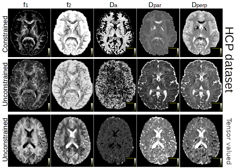
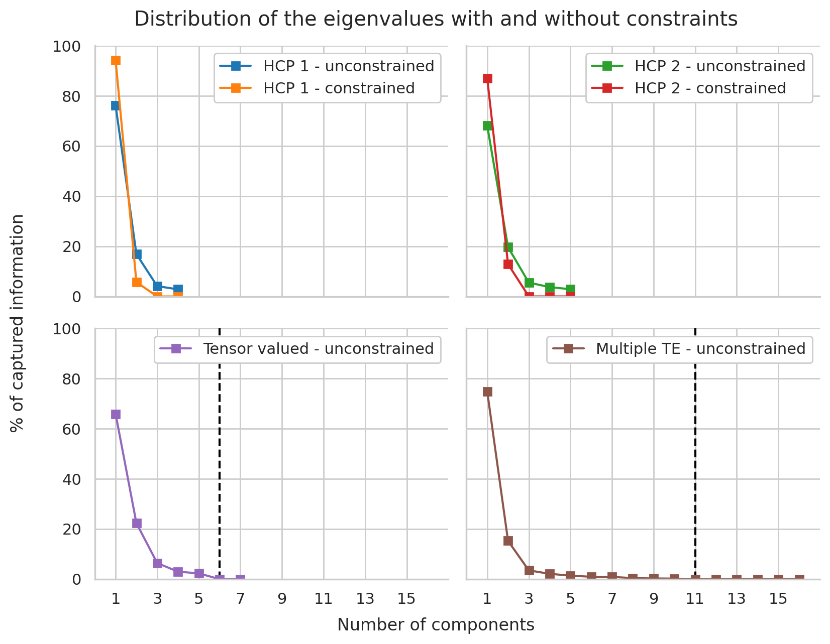
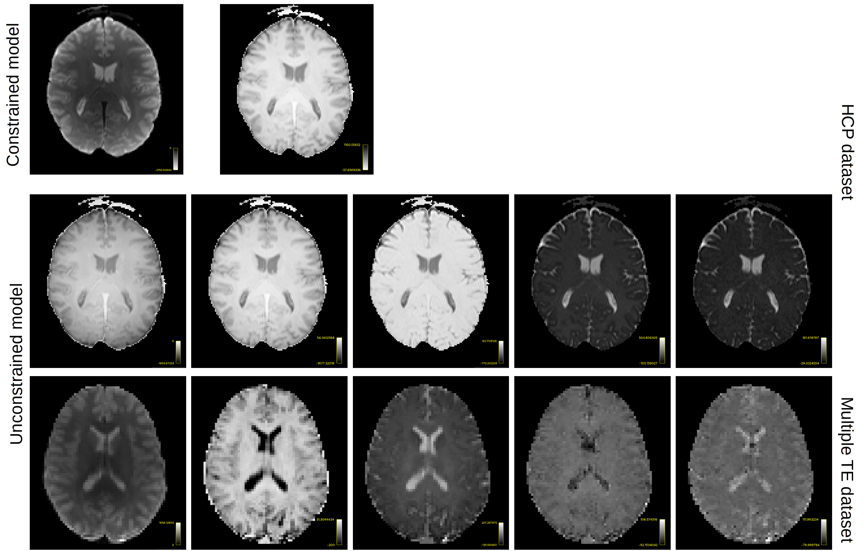
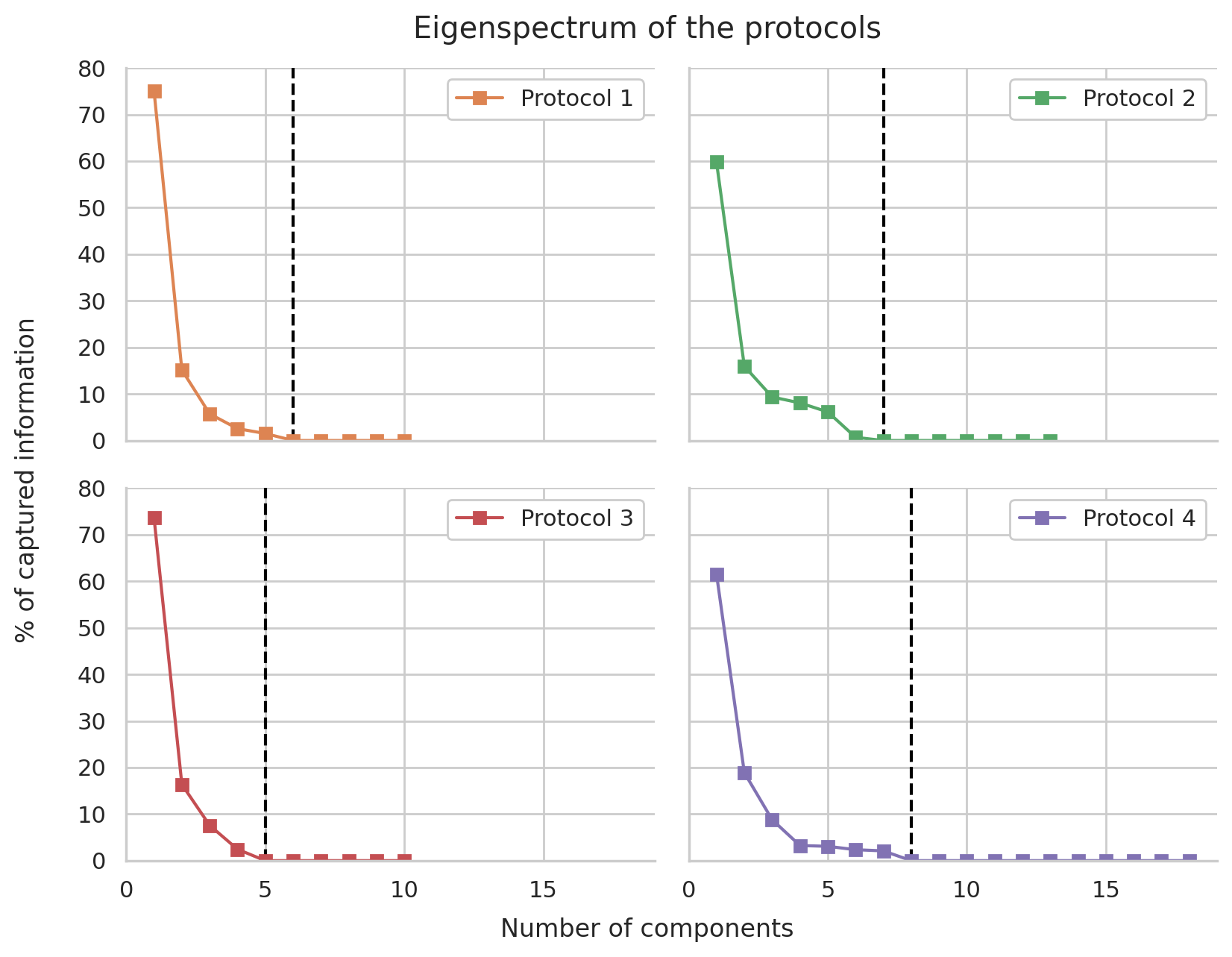
Figure 1 shows the obtained parameter maps for the HCP dataset and for the b-tensor dataset. The extra acquisition dimension added by b-tensor encoding stabilizes the estimated values of the model without constraining the solution. As shown in Figure 2, constraining Equation 2 improves the visual appearance of the result by projecting the model to a 2D subspace. The full model is supported by b-tensor encoding and multiple TEs as the eigenvalues for these models now reach zero. Figure 3 shows the first eigenvectors of the model for the HCP dataset and for the multiple TE dataset. The unconstrained model seems to capture similar information to the constrained model as evidenced by the similarity between their eigenvectors, but adding b-tensor encoding and multiple TEs shows additional variability in the first few eigenvectors. Figure 4 shows the eigenvalues of the model for different acquisition with multiple TEs and b-tensor shapes. In general, the information is spread out in multiple dimensions, but for the studied model the acquisition could be improved by projecting the data equally on the first few components and avoiding sharp decays in the eigenvalues.

Discussion and Conclusion

We have shown how the ideas of MRF can be leveraged to rapidly fit and analyze diffusion MRI models. This approach benefits from lesser computational hurdles than least-square fitting since a sequence of convex problems is solved separately for each signal compartment, independent of the signal fractions as shown in Equation 1. Projecting the data to another space with the SVD also enables visualization of the information contained in an acquisition protocol for a given model. This facilitates investigation of the adequacy of various models for a given acquisition scheme, or designing an optimal acquisition for a model of interest given a limited acquisition time. Future work will investigate how to incorporate information from the orientation distribution function (ODF) into the framework.

Acknowledgements

We would like to thank Chantal M.W. Tax and Beatrice Lena from the UMC Utrecht for ideas and suggestions.

Samuel St-Jean is supported by the Natural Sciences and Engineering Research Council of Canada (NSERC) [funding reference number BP–546283–2020] and the Fonds de recherche du Québec - Nature et technologies (FRQNT) [Dossier 290978].

Data were provided in part by the Human Connectome Project, MGH-USC Consortium (Principal Investigators: Bruce R. Rosen, Arthur W. Toga and Van Wedeen; U01MH093765) funded by the NIH Blueprint Initiative for Neuroscience Research grant; the National Institutes of Health grant P41EB015896; and the Instrumentation Grants S10RR023043, 1S10RR023401, 1S10RR019307.

Data were provided in part by the Human Connectome Project, WU- Minn Consortium (Principal Investigators: David Van Essen and Kamil Ugurbil; 1U54MH091657) funded by the 16 NIH Institutes and Centers that support the NIH Blueprint for Neuroscience Research; and by the McDonnell Center for Systems Neuroscience at Washington University.

References

1. Novikov, D. S.et al. (2018). Rotationally-invariant mapping of scalar and orientational metrics of neuronal microstructure with diffusion MRI. NeuroImage, 174, 518–538.

2. Ma, D., et al. (2013). Magnetic resonance fingerprinting. Nature, 495(7440), 187–192.

3. Eriksson, S. et al. (2015). NMR diffusion-encoding with axial symmetry and variable anisotropy: Distinguishing between prolate and oblate microscopic diffusion tensors with unknown orientation distribution. The Journal of Chemical Physics, 142(10), 104201.

4. Kaden, E., et al. (2016). Multi-compartment microscopic diffusion imaging. NeuroImage, 139, 346–359.

5. Fan Q, et al. Investigating the capability to resolve complex white matter structures with high b-value diffusion magnetic resonance imaging on the MGH-USC Connectom scanner. Brain Connect 2014;4(9):718-726.

6. Van Essen, D.C. et al, 2012. The Human Connectome Project: a data acquisition perspective. Neuroimage 62 (4), 2222–2231

7. Lampinen, B. et al.(2020). Towards unconstrained compartment modeling in white matter using diffusion‐relaxation MRI with tensor‐valued diffusion encoding. Magnetic Resonance in Medicine, 84(3), 1605–1623.

Figures

Figure 1: Parameter maps (diffusivities in mm²/s) obtained with maximizing the inner product for the two HCP datasets (top and middle row) and for the b-tensor dataset (bottom row). The constrained estimation (top row) enforces D_par > D_perp, leading to coherent-looking parameter maps by forcing the model into a lower dimensional space, which is not supported as well by the unconstrained version. The b-tensor encoded dataset suffers less from this degeneracy by providing an additional sample dimension.

Figure 2: Distribution of the eigenvalues for each dataset. The top row shows that constraining the model forces the parameters into a lower dimensional subspace supported by the data. This is not the case for the unconstrained version as the spectra do not decay to 0. In the bottom row, the black line indicates where the eigenvalues are zero, indicating that the model can be fully represented by the acquisition.

Figure 3: The first eigenvectors for the HCP dataset and for the multiple TE dataset. The constrained model is described by 2 components, despite being a four-parameter model. The first 5 eigenvectors of the unconstrained model show little contrast among themselves, suggesting that the acquisition cannot disentangle all model parameters. Bottom row shows the eigenvectors for data with varying b-tensors and TE. The contrast between images shows that additional information is captured by the acquisition.

Figure 4: Eigenvalues of the four protocols, where the black line indicates the first zero eigenvalue. An optimal acquisition would spread the information from the first N values equally into each of the N parameters of the model, indicating no linear relationship between the acquisition dimension. Protocol 4 can access more information than the others, but decays quicker than protocol 2. This may make protocol 4 more susceptible to noise and artifacts of the acquisition than protocol 2.

Proc. Intl. Soc. Mag. Reson. Med. 29 (2021)

2603