Introduction

Chemical exchange saturation transfer (CEST) is an emerging MRI technique that amplifies the detectability of certain low-concentration biomolecules through their interaction with the abundant water pool.^1,2 However, its routine clinical use is limited by the relatively long scan time since CEST MRI acquires multiple image frames.^3,4 Recently, a variably-accelerated SENSE (vSENSE) method was proposed to speed up the CEST acquisition.^5,6 Here, we propose a novel auto-calibrated reconstruction method by joint k-space and image-space parallel imaging (KIPI) as a further development of the vSENSE approach.

Theory

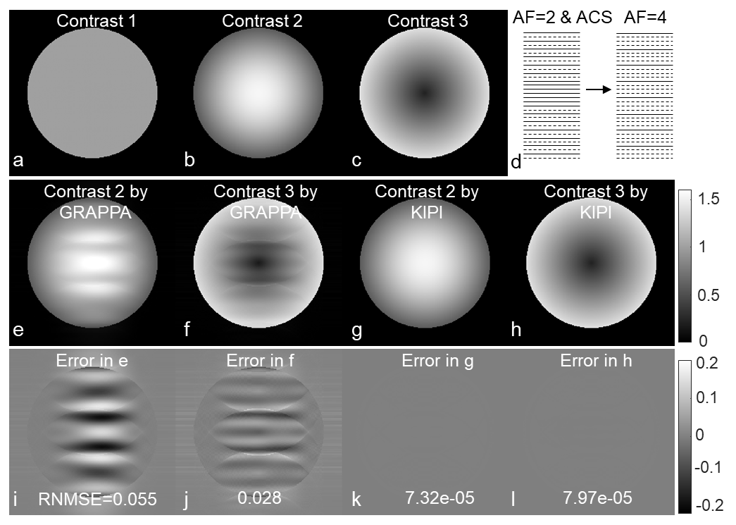
As an auto-calibrated k-space reconstruction method, GRAPPA⁷ estimates the missing k-space point by a linear combination of the acquired data in the neighborhood from all channels using the following equation,$$\begin{equation}y=Aw\tag{1} \end{equation}$$where $$$A$$$ represents the source matrix organized from the auto-calibration signal (ACS) data, $$$y$$$ denotes the target matrix, and $$$w$$$ represents the weights to be fitted. GRAPPA generates accurate images robustly when the acceleration factor (AF) is low.⁸ However, the GRAPPA weights estimated can be affected by the underlying image contrast. Figure 1 shows images of different contrasts simulated according to Biot-Savart law⁹ with eight receive channels. It is clear that the GRAPPA weights calculated from one contrast yield significant errors when being applied to the other contrasts (Figs. 1e-1f and 1i-1j).

SENSE¹⁰ poses the reconstruction as a linear inverse problem in image space and theoretically yields the optimal solution. However, the accuracy of SENSE reconstruction depends on the accuracy of the sensitivity maps used, which are prone to errors in practice.^5,6 If the coil image $$$m_{i}$$$ of channel $$$i$$$ ($$$1\leq i\leq N$$$) is perfectly known, the sensitivity map $$$SE_{i}$$$ can be obtained by dividing the coil-combined image $$$\rho$$$ into the image from each channel.$$\begin{equation}SE_{i}=m_{i}/\rho\tag{2}\end{equation}$$
Thus, for retroactive SENSE reconstruction with AF=2 (without loss of generality), there is $$\begin{equation}\begin{split}\begin{aligned}s_{N*1}&=m_{N*1}^{1}+m_{N*1}^{2}\\&=\rho^{1}SE_{N*1}^{1}+\rho^{2}SE_{N*1}^{2}\\&=\left[\begin{array}{ll}SE_{N*1}^{1}&SE_{N*1}^{2}\end{array}\right]\left[\begin{array}{l}\rho^{1}\\\rho^{2}\end{array}\right]\end{aligned}\end{split} \tag{3}\end{equation}$$ where $$$s_{N*1}$$$ represents the folded coil image vector, and the superscript represents the spatial position. The least squares solution to Eq. [3] is$$\begin{equation}\begin{split}\begin{aligned}\left[\begin{array}{c}\hat{\rho}^{1}\\\widehat{\rho}^{2}\end{array}\right]&=\left(SEE^{H}SEE\right)^{-1}SEE^{H}s_{N*1}\\&=\underbrace{\left(SEE^{H}SEE\right)^{-1}SEE^{H}SEE}_{I}\left[\begin{array}{l}\rho^{1}\\\rho^{2}\end{array}\right]=\left[\begin{array}{l}\rho^{1}\\\rho^{2}\end{array}\right]\end{aligned}\end{split} \tag{4}\end{equation}$$ where $$$SEE=\left[\begin{array}{ll}SE_{N*1}^{1}&\left.SE_{N*1}^{2}\right]\end{array}\right.$$$ and $$$I$$$ is the identity matrix.

However, the coil image $$$m_{i}$$$ is unknown for SENSE imaging with AF > 1 in practice. The KIPI method calculates $$$m_{i}$$$ with GRAPPA reconstruction from a low-AF calibration frame. Then, the sensitivity maps can be calculated with Eq. [2], and be applied to the other frames with high-AF SENSE reconstruction. Notably, the derivation above (Eqs. [2-4]) illustrates that the SENSE solution using the sensitivity maps derived from the calibration frame itself is identical to its GRAPPA solution.

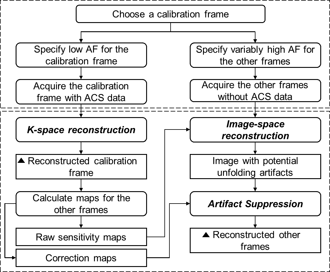
Overall, KIPI turns the original vSENSE approach into an auto-calibrated parallel imaging method by incorporating both GRAPPA and SENSE reconstruction. During data sampling, KIPI chooses an image frame as the calibration frame with low AF with the ACS data, and undersamples the other image frames using variably high AF without ACS data. During reconstruction, KIPI inherits the robustness of auto-calibrated GRAPPA imaging, and avoids the drawback of its susceptibility to underlying contrasts by calculating sensitivity maps. Furthermore, KIPI can adopt the artifact suppression algorithm used in vSENSE.^5,6 The KIPI approach is summarized in Figure 2.

Methods

Human experiments were conducted on a 3T Siemens Prisma MRI system using a 64-channel-receive head coil. A SPACE-CEST sequence¹¹ was run using the following readout parameters: FOV=212×212×201mm³, resolution=2.8×2.8×2.8mm³, turbo factor=140, and GRAPPA factor=2×2 with ACS acquired. Seven CEST saturation offsets for APT-weighted (APTw) imaging were executed, including (S0), ±3, ±3.5, and ±4-ppm. And a dual-echo 3D GRE sequence was used for B0 field mapping.

For retrospective reconstruction, the +3.5-ppm frame was selected as the calibration frame with AF=2×2 to generate the sensitivity maps and correction maps, and the remaining 6 frames had AF=2×4 (in the phase-encoding and partition-encoding directions, respectively). Note that only the calibration frame retained ACS data.

Results

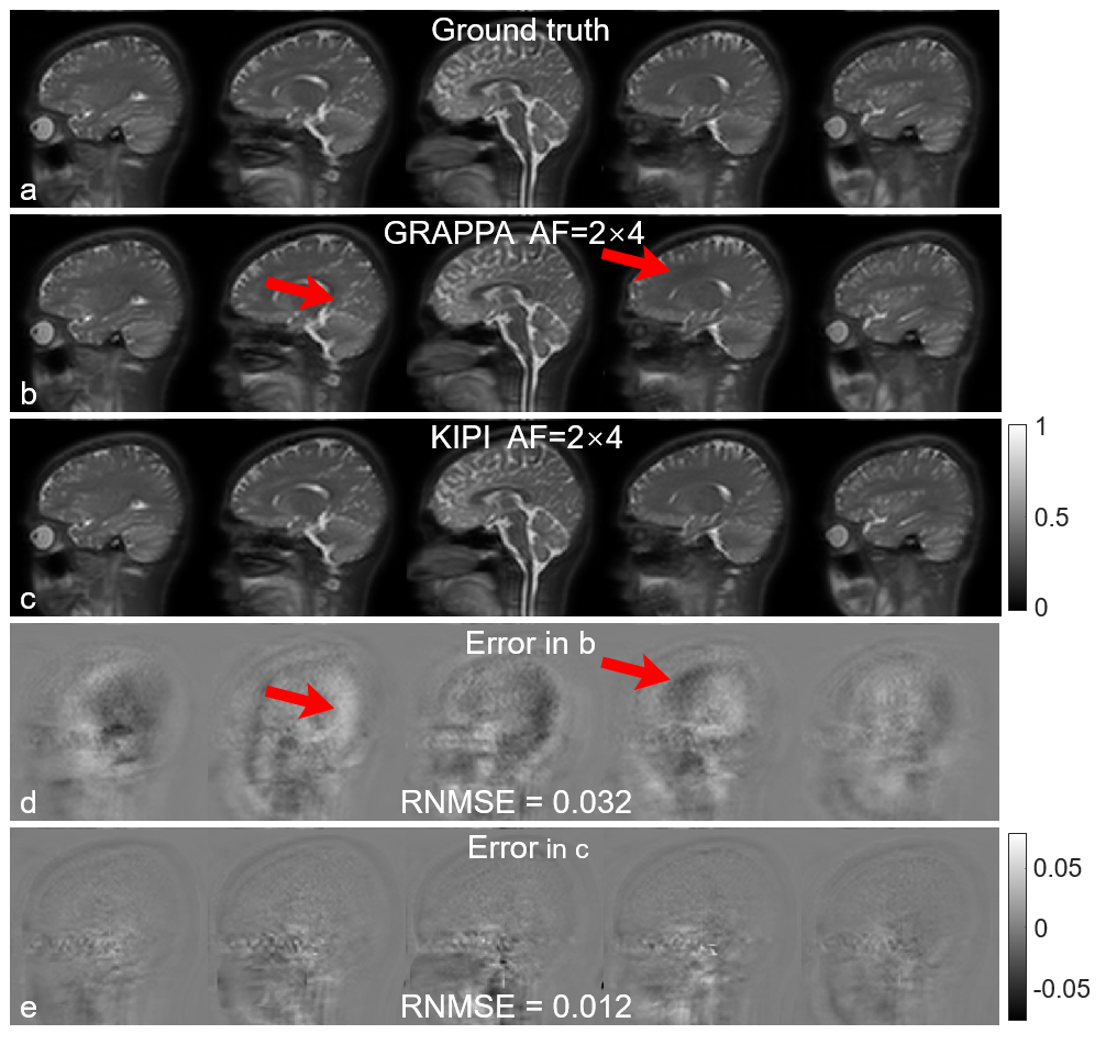
Figures 1g-h show KIPI allowed a calibration frame with a different image contrast to be used, generating reconstruction errors substantially smaller than those from GRAPPA (Figs. 1k-l vs. 1i-j). On the contrary, the accuracy of GRAPPA was comprised when reusing the kernel weights across different image contrasts (Figs. 1e-f).

The conventional GRAPPA (AF=2×2) scan (Fig. 3a) was considered ground truth here. KIPI (Fig. 3c) generated source images that better agreed with the ground-truth results than those reconstructed from GRAPPA (Fig. 3b) using the same data (AF=2×4) with RNMSE of 0.012 versus 0.032, respectively. Besides, unfolding artifacts were evident in the GRAPPA images (Figs. 3b, d; red arrows).

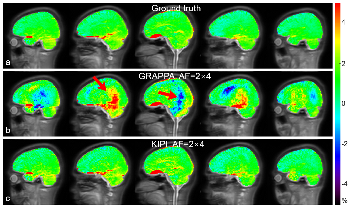
Figure 4 displays the APTw images calculated from the source images of Fig. 3 after B0 correction and image alignment. Substantial artifacts can be seen in the APTw images reconstructed by GRAPPA (Fig. 4b) while the KIPI method generated APTw maps (Fig. 4c) that were consistent with the ground truth (Fig. 4a).

Conclusion

KIPI is a novel auto-calibrated parallel imaging method that incorporates the advantages of k-space and image-space reconstruction methods. KIPI allowed an acceleration factor of up to 8-fold for acquiring CEST source images, yielding a net speed-up of 6-fold in scan time, and essentially without compromising the image quality. KIPI should facilitate the translation of CEST imaging in clinical routines.

Acknowledgements

NSFC grant number: 81971605, 61801421.