2592

Joint and individual statistical analysis of brain MRI and cognition measures in Alzheimer's Disease

Raphiel Jamale Murden¹, Deqiang Qiu², and Benjamin B Risk²
¹Biostatistics and Bioinformatics, Emory University, Atlanta, GA, United States, ²Emory University, Atlanta, GA, United States

Synopsis

Canonical Joint and Individual Variation Explained (CJIVE) provides a method for jointly analyzing multi-block datasets collected from the same individuals. We apply this method to measures of brain morhometry and cognition from a sample of older adults. We found latent patterns of joint variation across data types which were statistically associated with diagnoses of Alzheimer's Disease and mild cognitive impairment. We also found that the unique patterns of variation within each data type were not associated with diagnoses.

Introduction

Alzheimer’s Disease is associated with changes that can be measured using multiple modalities such as cognitive assessment and brain volumetry using MRI. Data integration methods, such as the classic Hotelling's canonical correlation analysis (CCA)¹ can find shared or joint structure across multiple datasets/modalities (i.e. data blocks, data matrices). More recent approaches include multiset Canonical Correlation Analysis or M-CCA², Joint and Individual Variance Explained (JIVE)³, Angle-based JIVE (AJIVE)⁴, and others. The JIVE framework decomposes each of two or more data blocks into a joint subspace shared across all blocks, an individual subspace that is unique to each data block, and noise. Here, individual refers to signal unique to a dataset. However, interpreting these subspaces remains challenging. To aid interpretation, we propose an alternative view of the JIVE decomposition and provide an updated estimation method called Canonical JIVE or CJIVE. We apply CJIVE to measurements of brain morphometry and cognition from The Alzheimer's Disease Prediction of Longitudinal Evolution (TADPOLE) Challenge⁵.

Methods

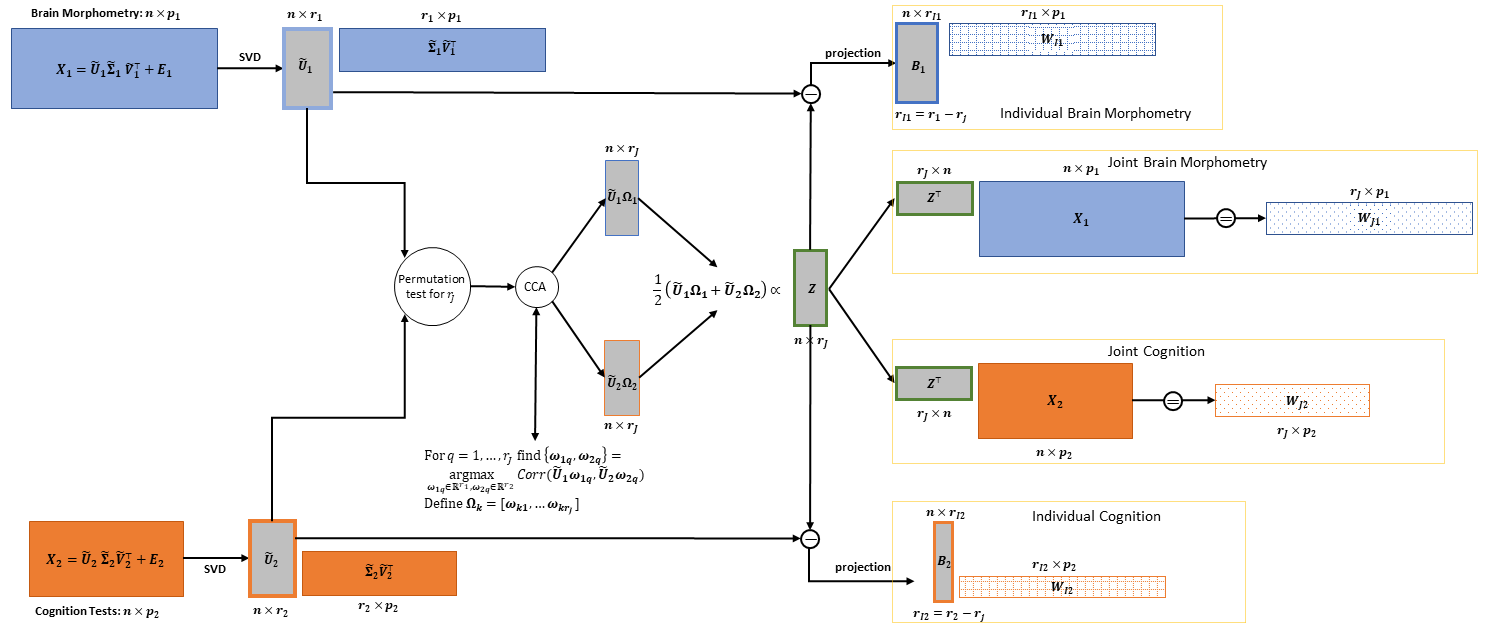
Figure 1 illustrates the CJIVE decomposition methodology. The first step involves the principal component analysis (PCA) of each data block for cognitive functions and MRI measures separately. CCA is then applied to the left singular vectors (i.e. principal component (PC) scores), with the number of canonical variables, $$$r_J$$$ determined by a permutation test. Each joint component’s subject score $$$Z_i$$$ is an average of the $$$i^{th}$$$ canonical variables. Joint subject scores can then be used to obtain joint variable loadings, $$$W_{Jk}$$$, and then the orthogonal complement of the joint subspace intersected with the PC subspace from the first step is used to obtain individual subject scores, $$$B_k$$$ and individual loadings $$$W_{Ik}.$$$ The approach has similarities to M-CCA, except that 1) JIVE estimates both joint structure and individual structure, whereas CCA discards individual structure; 2) the JIVE model provides a more parsimonious summary of the joint structure as a joint subspace, rather than the data-specific subspaces of CCA; and 3) the JIVE estimate will be more accurate when there exists a shared subject score subspace⁴. Compared to AJIVE⁴, we a) propose a novel use of probabilistic Principal Components Analysis (pPCA)⁶ for subject score imputation in the presence of missing data and b) develop a computationally efficient permutation test for joint structure.

We applied CJIVE to data obtained from 1400 participants in the TADPOLE Challenge taken at their 6-month follow-up visit. The variables of interest were divided into two groups: brain morphometry measures and cognition measures. The morphometry measures consist of 205 cortical volume, cortical thickness, and surface area measurements for regions of interest (ROIs) determined by the Desikan-Killany brain atlas⁷. The cognition measures comprise 22 scores and sub-scores from seven validated scales. However, 15 of these were missing for nearly 60% of the participants. In the first step of CJIVE analysis, we use pPCA to impute the missing values and obtain PC scores. To avoid confounding, the input datasets consist of residuals after regressing out age and sex. We also examined four-way JIVE treating volume, cortical thickness, surface area, and cognition as separate datasets, but the two-way JIVE led to better grouping by diagnosis and is presented below.

Results

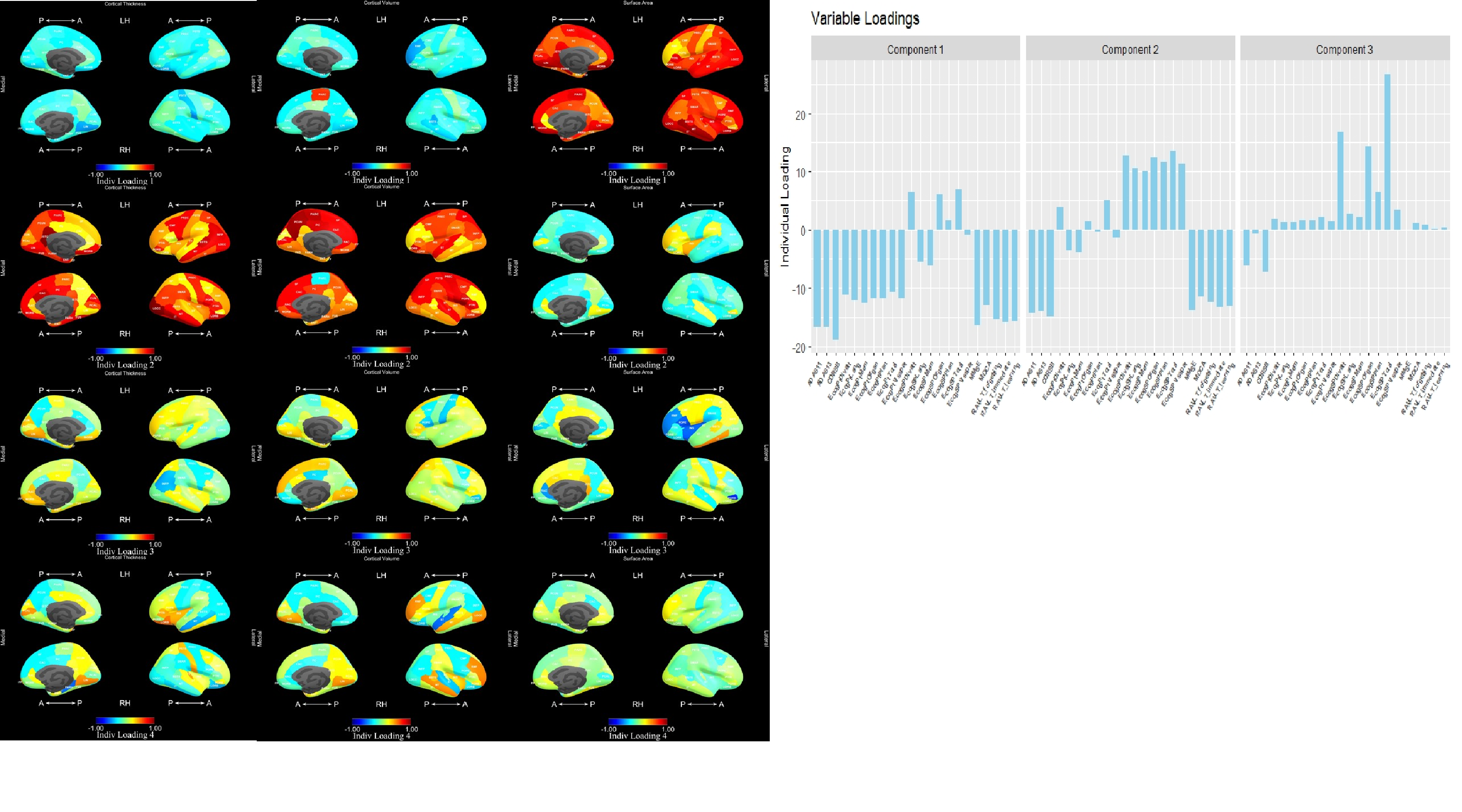
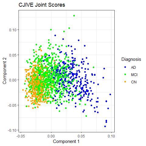
CJIVE found $$$r_J = 2$$$ joint components between cognition and brain morphometry measures. Figure 2 shows a clear clustering of scores by diagnosis for component 1, but not component 2. However, one may note that a much smaller proportion of cognitively normal (CN) participants had component 2 scores that fell outside of the range (-0.05, 0.05) when compared to participants diagnosed with mild cognitive impairment (MCI) or Alzheimer's disease (AD). We examined the utility of joint scores as possible disease discriminant factors by performing logistic regression. Both joint subject score components were statistically significant predictors of the log-odds of an MCI diagnosis compared to CN and MCI compared to AD $$$(p<0.001)$$$.

For the first component joint loadings, Figure 3 shows that most cognitive measures, except for the Forgetting subscale of the Rey Auditory Verbal Learning Test (RAVLT)⁸ and Everyday Cognition (Ecog) patient (PT) subscales⁹, correspond strongly with measures of cortical thickness in several regions and cortical volume in a few regions of the temporal lobe. There was also strong left-right symmetry in both cortical thickness and volume. Additionally, entorhinal cortical thickness was prominent. In contrast to cortical thickness and volume, surface area was a minor source of joint information.

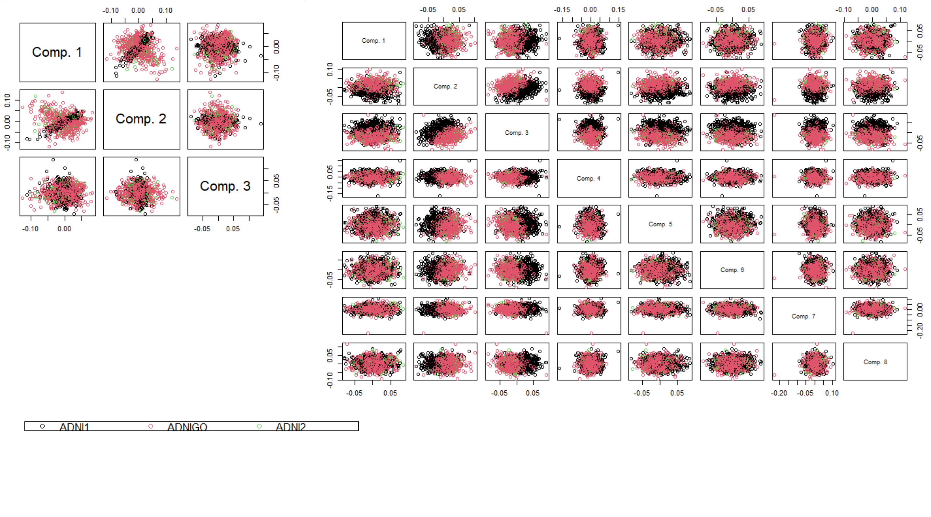
Individual cognition scores were weakly associated with diagnosis, while morphometry scores were not associated. However, we found they were associated with the ADNI phase during which a subject's data were collected (Figure 4). As for loadings (Figure 5), in the first individual morphometry component, measurements of surface area dominated while thickness and volume measures were prominent in the second component. However, few components displayed strong left-right symmetry as in the joint subspace.

Discussion and conclusion

Since joint scores were associated with diagnosis and individual scores with ADNI phase, the sources of variation that differentiate diagnoses seem consistent across study phases even if other factors are not. Joint loadings point to morphometry measures that vary with cognition measures. CJIVE provides a powerful method for the decomposition of information in MRI and other types of measurements into shared and unique components.

Acknowledgements

The project was supported by a Pilot grant from the Goizueta Alzheimer’s Disease Research Center at Emory University (NIH P50 AG025688).

References

1. Hotelling, H. (1936). Relations Between Two Sets of Variates. Biometrika, 28(3/4), 321-377. doi:10.2307/2333955

2. Li, Y. O., Adali, T., Wang, W., & Calhoun, V. D. (2009). Joint blind source separation by multiset canonical correlation analysis. IEEE Transactions on Signal Processing, 57(10), 3918-3929.

3. Lock, E. F., Hoadley, K. A., Marron, J. S., & Nobel, A. B. (2013). Joint and individual variation explained (JIVE) for integrated analysis of multiple data types. The annals of applied statistics, 7(1), 523.

4. Feng, Q., Jiang, M., Hannig, J., & Marron, J. S. (2018). Angle-based joint and individual variation explained. Journal of multivariate analysis, 166, 241-265.

5. Marinescu, R. V., Oxtoby, N. P., Young, A. L., Bron, E. E., Toga, A. W., Weiner, M. W., ... & Alexander, D. C. (2018). Tadpole challenge: Prediction of longitudinal evolution in Alzheimer's disease. arXiv preprint arXiv:1805.03909.

6. Tipping, M. E., & Bishop, C. M. (1999). Probabilistic principal component analysis. Journal of the Royal Statistical Society: Series B (Statistical Methodology), 61(3), 611-622.

7. Desikan, R. S., Ségonne, F., Fischl, B., Quinn, B. T., Dickerson, B. C., Blacker, D., ... & Albert, M. S. (2006). An automated labeling system for subdividing the human cerebral cortex on MRI scans into gyral based regions of interest. Neuroimage, 31(3), 968-980.

8. Rey, A. (1941). The Rey Auditory Verbal Learning Test. L’examen psychologique dans les cas d’encéphalopathie traumatique. Arch Psychol (Geneve), 28, 286-340.

9. Farias, S. T., Mungas, D., Harvey, D. J., Simmons, A., Reed, B. R., & DeCarli, C. (2011). The measurement of everyday cognition: development and validation of a short form of the Everyday Cognition scales. Alzheimer's & Dementia, 7(6), 593-601.

Figures

Schematic of the CJIVE process. Singular value decomposition (SVD) is applied to the input data matrices (far left) to obtain dimension-reduced PC scores. Next, a permutation test is used to determine the number of components that will lie in the joint subspace. CCA is applied to the PC scores and a weighted average of canonical variables determines the joint subspace. Finally, individual subspaces can be determined by the orthogonal complement of the joint subspace within the respective PC subspaces.

Scatterplot of joint subject scores colored by diagnosis with component 1 along the x-axis, and two along the y-axis. For component 1, participants diagnosed with AD tend to have higher scores than those with mild cognitive impairment (MCI). Similarly, participants with MCI (mild cognitive impairment) tend to have higher scores than CN (cognitively normal) participants. Extreme values in the second component tend to be associated with either MCI or AD.

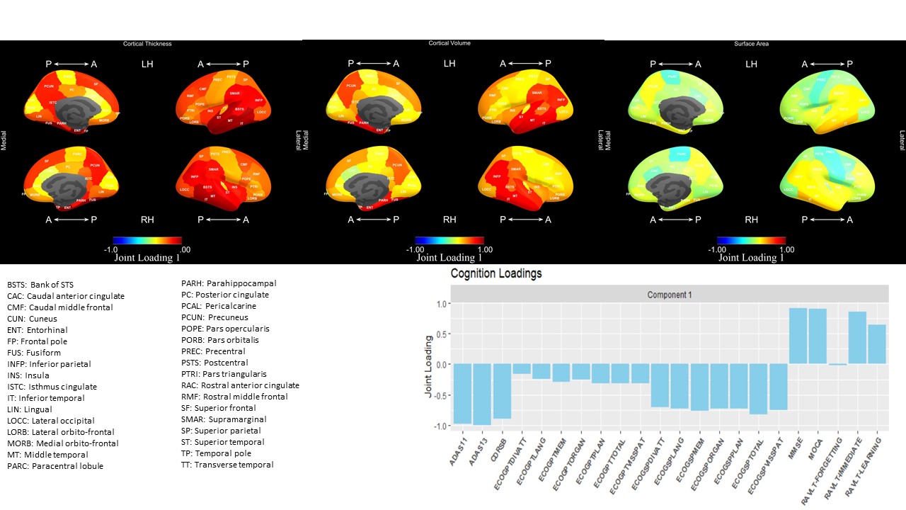
Joint Loadings for component 1. Temporal lobe ROI measures were most prominent among morphometry loadings, including both thickness and volume. ADAS and MMSE dominated cognition loadings (bottom) and both have been shown as excellent diagnostic tools. The proportions of total variation explained by the first joint component were 0.147 for morphometry and 0.467 for cognition. Proportions explained by the second component (not shown) were 0.025 and 0.044 for morphometry and cognition, respectively.

Individual subject scores for each dataset, colored by the ADNI phase during which the participant's 6-month follow-up data were collected. Morphometry components 2 and 3 each cluster by ADNI phase. A strong linear relationship exists between cognition components 1 and 2 for participants from the ADNI1 phase. For ADNI2 and ADNIGO participants, the same relationship goes in the opposite direction and is weaker.

Individual variable loadings for each dataset. Loadings were most prominent for surface area measurements in the first individual morphometry component. Cortical thickness and volume measures dominated the second and third loadings. The proportions of variation explained by individual morphometry components were 0.14 and 0.11 in the first two, respectively, and less than 0.04 for the remainder (3-8). For cognition, the proportions were 0.13, 0.10, and 0.06, respectively.

Proc. Intl. Soc. Mag. Reson. Med. 29 (2021)

2592