2493
GPU accelerated calculations of the scattered RF-field due to a dielectric update without extensive pre-calculated data.1Computational Imaging, UMC Utrecht, Utrecht, Netherlands, 2Biomedical Engineering, Eindhoven University of Technology, Eindhoven, Netherlands
Synopsis
Previous work showed that the scattered RF-fields created by dielectric pads and medical implants can quickly be calculated. The method requires an extensive offline calculation stage and a lot of memory. We propose an extension to the method that removes these two problems by using a volume integral equation solver. This allows us to do the entire calculation on a GPU for more acceleration. The resulting scattered electric fields have a maximum difference of 3.2% with respect to FDTD, while currently being a 106 times faster. Eventually, we want to use this method for patient-specific implant RF-safety assessment.
Introduction
The scattered RF-field created by high permittivity dielectric pads and medical implants can be quickly calculated as shown in1,2.The method updates the incident RF-fields from the RF coil to include the dielectric properties of the pad/implant. This update replaces any existing dielectric that is present in the simulation with that of the pad/implant. The fast calculation is achieved by exploiting the fact that the pad/implant occupies only a small volume within the entire domain of the RF-coil and the patient anatomy.
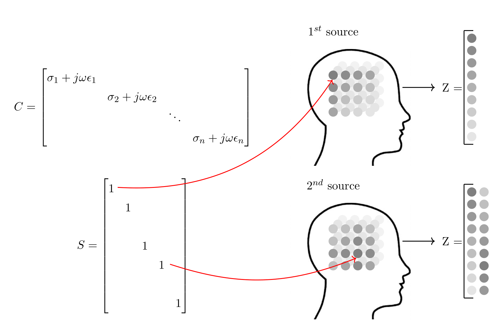
The equation that is solved to do this is$$E^t=E^i+Z(I-CS^TZ)^{-1}CS^TE^i\,\,\,\,\,\,\,\,\,(1)$$where $$$E^t$$$ is the total electric field (with implant), $$$E^i$$$ is the incident electric field (without implant) and $I$ is the identity matrix. The other quantities are illustrated in Figure 1.
The library matrix $$$Z$$$ consists out of a set of single edge source simulations which has $$$M$$$ by $$$N$$$ values with $$$M$$$ being all the voxel edges within the entire simulated domain (i.e. RF-coil and patient) and $$$N$$$ the number of voxel edges within the update domain (i.e. only the implant or pad). For realistic resolutions used for patient simulations, the library matrix becomes intractable and too large to fit inside the memory of a computer. For example, if a 15x15x15 cm3 volume within the human brain needs to be stored at a 1x1x1 mm3 resolution the library matrix would be 746TB large using single-precision complex values.
In this work, we propose an online calculation method that does not require the library matrix. We replace the library matrix with a function using the volume integral equation (VIE) that calculates only the resultant electric field3. This allows us to run the entire problem on a GPU for more acceleration because the memory requirements are significantly reduced.
Methods
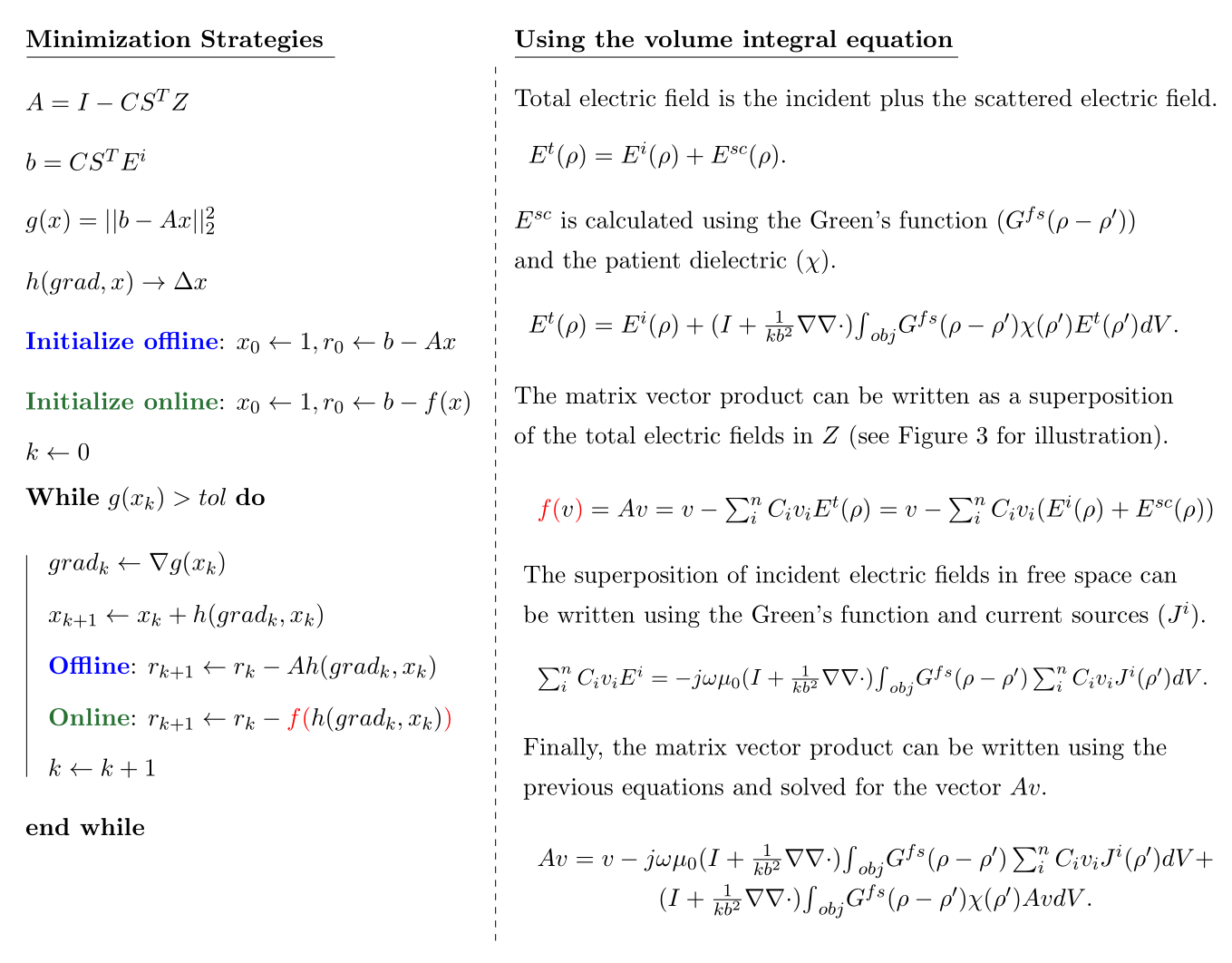
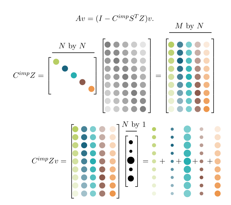
In Figure 2 we show the minimization process used to solve Equation 1 and how we replace the need for the library matrix, contained inside $$$A$$$. We instead formulate a function that calculates the matrix-vector product of $$$A$$$ with some vector $$$v$$$.This is done with the VIE using a superposition of $$$N$$$ sources located at the edges of the dielectric updates. This principle is illustrated in Figure 3. We show that using this VIE formulation we can calculate the product of the library matrix with the found current density and that we can solve Equation 1 using this formulation.
We used Duke from the virtual family (IT'IS, Zurich Switzerland)4 and FDTD simulations using Sim4Life (ZMT, Zurich Switzerland) to compare with the proposed method, which is implemented in the Julia programming language using CUDA.jl to compute the VIE on a GPU5,6. Furthermore, we compare our old method using the library matrix explicitly (offline method) against the current method that uses the function based on the VIE (online method).
Results
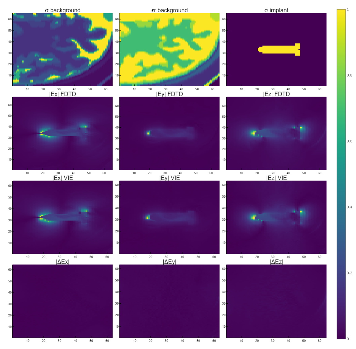
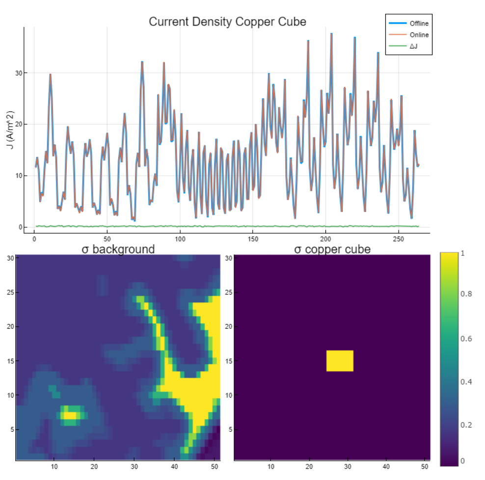
In Figure 4 the result of the library matrix times a known current density is shown to demonstrate the validity of the proposed method. This result was obtained within 0.1 seconds on an NVidia RTX 2070 Super and has a maximum absolute error of 3.17%.Equation 1 has also been solved for a small dielectric update (a copper cube) using the proposed online method. This result was obtained in 34 seconds on the same GPU. The simulation using an FDTD solver took 1 hour, which is about 106 times faster. The code for the solver of Equation 1 is not optimized yet so there is still some acceleration to be obtained. Furthermore, this method could be combined with previous work that we showed using a physics-based neural network to increase the acceleration further.
Discussion & Conclusion
Using the proposed method the library matrix is no longer required to be known explicitly. This removes a large burden that this method was suffering from, which is the memory required to store this library matrix. Furthermore, the offline calculation phase where the simulations for the different columns in the library matrix are computed is not necessary. Moreover, a patient-specific dielectric can be used for the simulation of the scattered electric field. Before, the library matrix needed to be computed using one of the virtual family members. This change will reduce inter-subject variations in the electric field.A downside of using the proposed method is that it is slower than the offline method because at every iteration of the minimization process a forward simulation is done to obtain the required matrix-vector product. Furthermore, at a certain number of edges $$$N$$$ solving Equation 1 becomes slower than running a new FDTD simulation. However, this method does not suffer from the resolution of the voxelization. Thus, very small implants like aneurysm clips could quickly be simulated.
Currently, we are still working on the stability of the solver for Equation 1, as it fails to simulate larger dielectric updates with the same accuracy as shown here. Eventually, we want to use the proposed method for patient-specific implant RF safety assessment. Ideally, the type and the location of the implant are known, for example from x-ray images made of the implant after placement, before the patient comes in.
Acknowledgements
No acknowledgement found.References
1. Van Gemert, J. H., Brink, W., Webb, A., & Remis, R. (2016). An efficient methodology for the analysis of dielectric shimming materials in magnetic resonance imaging. IEEE transactions on medical imaging, 36(2), 666-673.
2. Stijnman, Peter RS, et al. Accelerating implant RF safety assessment using a low‐rank inverse update method. Magnetic Resonance in Medicine, 2020, 83.5: 1796-1809.
3. Yla-oijala, Pasi, et al. Surface and volume integral equation methods for time-harmonic solutions of Maxwell's equations. Progress in electromagnetics Research, 2014, 149: 15-44.
4.Christ A, et al. The Virtual Family--development of surface-based anatomical models of two adults and two children for dosimetric simulations. Phys Med Biol. 2010 Jan 21;55(2):N23-38. doi: 10.1088/0031-9155/55/2/N01. Epub 2009 Dec 17. PMID: 20019402.
5. Bezanson, Jeff, et al. Julia: A fast dynamic language for technical computing. arXiv preprint arXiv:1209.5145, 2012.
6. Besard, Tim, et al. Effective extensible programming: unleashing Julia on GPUs. IEEE Transactions on Parallel and Distributed Systems, 2018, 30.4: 827-841.
Figures