2472
Multi-tissue log-domain intensity and inhomogeneity normalisation for quantitative apparent fibre density1Developmental Imaging, Murdoch Children's Research Institute, Melbourne, Australia, 2Florey Institute of Neuroscience and Mental Health, University of Melbourne, Melbourne, Australia, 3Centre for the Developing Brain, School of Biomedical Engineering and Imaging Sciences, King's College London, London, United Kingdom, 4Department of Biomedical Engineering, School of Biomedical Engineering and Imaging Sciences, King's College London, London, United Kingdom
Synopsis
Multi-tissue constrained spherical deconvolution of diffusion MRI data yields white matter fibre orientation distributions, from which a quantitative metric of apparent fibre density can be obtained. Unlike most other diffusion MRI models, this fibre density metric is directly proportional to the diffusion-weighted signal magnitude, and thus intensity normalisation and bias field correction are needed to compare it between subjects in a study. Here we propose an intensity and inhomogeneity correction algorithm for multi-tissue constrained spherical deconvolution results, estimating a bias field and global normalisation in the log-domain. It outperforms a previously proposed approach that did not operate in the log-domain.
Purpose
Constrained spherical deconvolution (CSD)[1] of diffusion MRI (dMRI) data results in white matter (WM) fibre orientation distributions (FODs), from which a quantitative metric of apparent fibre density (FD)[2] can be obtained. This FD metric is proportional to the (diffusion-weighted) signal, and is studied e.g. using the fixel-based analysis (FBA) framework[3,16]. This is unlike several other dMRI models that model signal relative to b=0 data, which ignores individually differing b=0 (T2) signal between model compartments[4,5]. However, quantitative studies of FD require intensity normalisation, to correct for both global and spatially inhomogeneous intensity variations (e.g. due to bias fields). Finding reliable reference areas is hard in the presence of unknown pathology, and bias field correction[6] using b=0 data is challenged due to limited contrast between WM and gray matter (GM).A solution to these challenges was proposed by Raffelt et al. in [7], by leveraging information from 3-tissue CSD techniques[8,9]. In this work, we aimed to improve upon that approach by:
- more accurately modelling bias fields as a multiplicative effect, which is typically achieved by performing estimation in the log-domain[10].
- adding an outlier rejection mechanism, to deal with locally less smooth variations of total (T2w) signal not accounted for in the model (not genuinely arising from bias fields).
We evaluate the performance using the same reference ground truth as Raffelt et al. in [7].
Methods
Similar to [7], our method assumes that all voxels in the brain are composed of a mixture of WM, GM and/or CSF; so most signal should generally be "accounted for". This means that the sum of all tissue compartment signals is expected to be close to 1, and hence also spatially relatively constant, with the exception of bias fields. Hence, the method ultimately aims to estimate a spatially smoothly varying intensity normalisation factor that, when applied to the total signal (sum of all tissues), brings it close to 1. To this end, three different things are jointly optimised; by estimating each one individually given the current estimation for the other two. These are:- Outlier rejection: the current total signal (sum of all tissues) is checked for outliers by calculating Tukey fences on the logarithm of the total signal.
- Tissue balance factors: due to specific scaling of individual tissue response functions, the sum of all tissues map might still show tissue contrast. This is minimised by computing a global balance factor for each tissue, constrained by requiring that all tissue balance factors multiply to 1.
- Spatially smooth normalisation field: the idea is that, when dividing the final total signal map by the final normalisation field, a value close to (spatially constant) 1 is obtained. To solve this multiplicative problem, we take the logarithm of both sides of the equation; i.e. when subtracting the logarithm of the final normalisation field from the logarithm of the total signal map, a value close to log(1)=0 should be obtained. The logarithm of the normalisation field is fitted as a cubic polynomial. Hence, the final normalisation field is the exponential of this polynomial.
Within the algorithm, the outlier rejection and tissue balance factors are optimised in an inner loop, by iterating both until convergence. This is followed by optimising the smooth normalisation field given current balance factors and excluding outliers. Both of these processes are iterated in the outer loop until convergence.
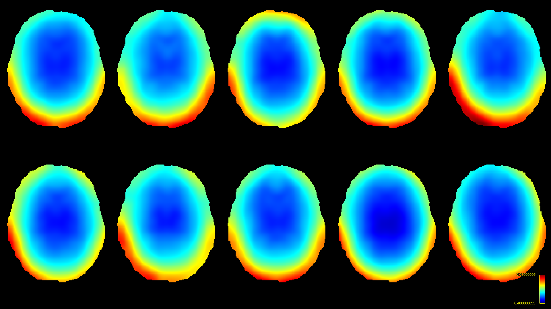
Both methods were implemented using MRtrix3[11] to compare performance. For this comparison, we reproduced the same software phantom approach as also used by Raffelt et al. in [7]. Briefly, this is a phantom derived by "Diffantom"[12] from human connectome project (HCP)[13] data. This phantom is a single-shell dataset with b=2000s/mm² for 128 gradient directions and a b=0 image. It has a voxel-size of 1.25×1.25×1.25mm³ and, crucially, features no intensity inhomogeneities by construction. Ten ground truth bias fields (Fig.1) from different HCP subjects were applied to the phantom. Single-shell 3-tissue CSD (SS3T-CSD)[9] was performed with 3-tissue response functions estimated from the data themselves[14,15]; using MRtrix3Tissue (https://3tissue.github.io/ ; a fork of MRtrix3[11]).
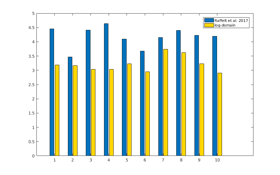
Intensity and inhomogeneity correction was then performed using both Raffelt et al. [7] and our proposed method. Performance was assessed by calculating relative (percent) error between total signal from the result after correction, and the original (unaffected) phantom.
Results and Discussion
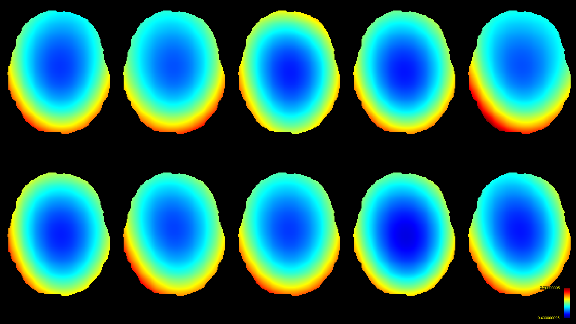
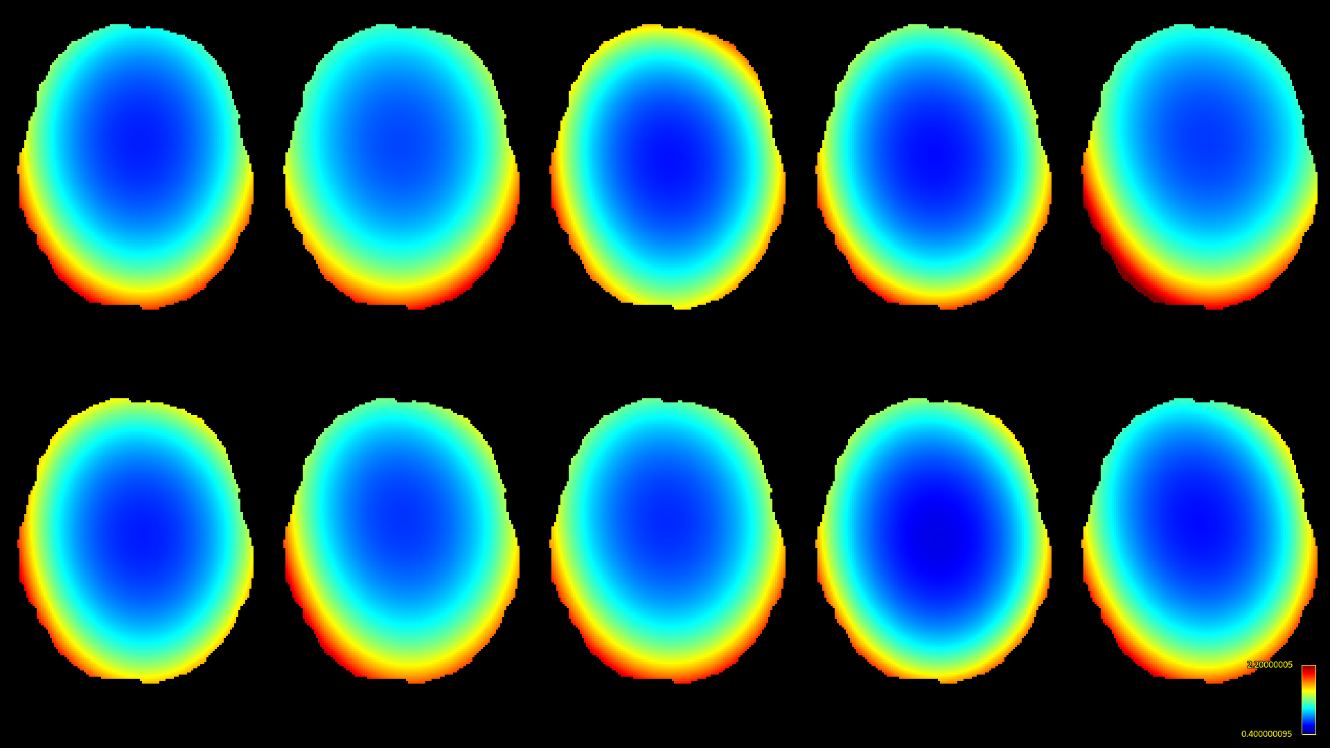
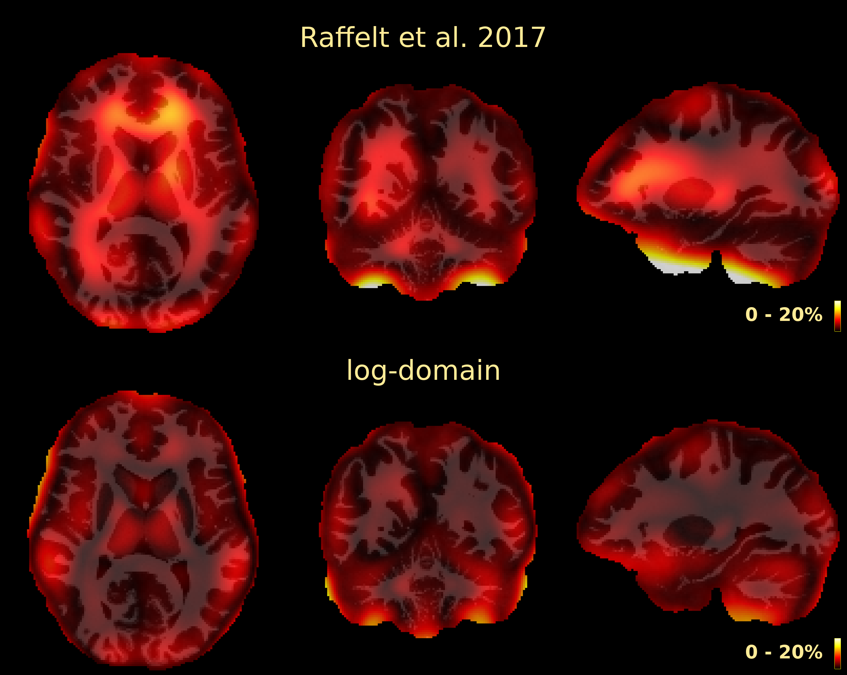
The resulting bias fields estimated by both methods are shown in Fig.2 and Fig.3, for comparison with the ground truth bias fields shown in Fig.1. The proposed log-domain method appears to consistently outperform the Raffelt et al.[7] method, as evidenced by lower relative errors (Fig.4). The Raffelt et al.[7] method appears to struggle mostly at extremities of the bias field value range (Fig.5). At some edges of the mask, this results in gradually escalating errors (Fig.5), beyond 20% and up to 35% in some voxels.Finally, note however that bias field correction and intensity normalisation of dMRI data is not relevant when studying (diffusion) signal fractions, as explicit normalisation to unity is implied in such approaches[17,18,19,20].
Conclusion
We propose an intensity and spatial inhomogeneity correction algorithm for multi-tissue constrained spherical deconvolution results, estimating a bias field and global normalisation in the log-domain. It outperforms a previously proposed approach that did not operate in the log-domain.Acknowledgements
No acknowledgement found.References
[1] Tournier JD, Calamante F, Connelly A. Robust determination of the fibre orientation distribution in diffusion MRI: Non-negativity constrained super-resolved spherical deconvolution. NeuroImage 2007;35(4):1459-1472.
[2] Raffelt D, Tournier JD, Rose S, Ridgway GR, Henderson R, Crozier S, et al. Apparent Fibre Density: a novel measure for the analysis of diffusion-weighted magnetic resonance images. NeuroImage 2012;59:3976-94.
[3] Raffelt D, Tournier JD, Smith RE, Vaughan DN, Jackson G, Ridgway GR, et al. Investigating white matter fibre density and morphology using fixel-based analysis. NeuroImage 2017;144:58-73.
[4] Bouyagoub S, Dowell NG, Hurley SA, Wood TC, Cercignani M. Overestimation of CSF Fraction in NODDI: Possible Correction Techniques and the Effect on Neurite Density and Orientation Dispersion Measures. In: Proc. Int. Soc. Magn. Reson. Proc ISMRM 2016;24:7.
[5] Berlot R, Metzler-Baddeley C, Jones DK, O’Sullivan MJ. CSF contamination contributes to apparent microstructural alterations in mild cognitive impairment. NeuroImage 2014;92:27-35.
[6] Tustison NJ, Avants BB, Cook PA, Zheng Y, Egan A, Yushkevich PA, Gee JC. N4ITK: Improved N3 bias correction. IEEE TMI 2010;29(6):1310-1320.
[7] Raffelt D, Dhollander T, Tournier JD, Tabbara R, Smith R, Pierre E, Connelly A. Bias Field Correction and Intensity Normalisation for Quantitative Analysis of Apparent Fibre Density. Proc ISMRM 2017;25:3541.
[8] Jeurissen B, Tournier JD, Dhollander T, Connelly A, Sijbers J. Multi-tissue constrained spherical deconvolution for improved analysis of multi-shell diffusion MRI data. NeuroImage 2014;103:411-426.
[9] Dhollander T, Connelly A. A novel iterative approach to reap the benefits of multi-tissue CSD from just single-shell (+b=0) diffusion MRI data. Proc ISMRM 2016;24:3010.
[10] Sled JG, Zijdenbos AP, Evans AC. A nonparametric method for automatic correction of intensity nonuniformity in MRI data. IEEE TMI 1998;17(1):87-97.
[11] Tournier JD, Smith R, Raffelt D, Tabbara R, Dhollander T, Pietsch M, Christiaens D, Jeurissen B, Yeh CH, Connelly A. MRtrix3: A fast, flexible and open software framework for medical image processing and visualisation. NeuroImage 2019;202:116137.
[12] Esteban O, Caruyer E, Daducci A, Bach-Cuadra M, Ledesma-Carbayo MJ, Santos A. Diffantom: Whole-Brain Diffusion MRI Phantoms Derived from Real Datasets of the Human Connectome Project. Front. Neuroinform 2016;4.
[13] Van Essen DC, Ugurbil K, Auerbach E, Barch D, Behrens TEJ, Bucholz R, et al. The Human Connectome Project: a data acquisition perspective. NeuroImage 2012;62:2222-2231.
[14] Dhollander T, Raffelt D, Connelly A. Unsupervised 3-tissue response function estimation from single-shell or multi-shell diffusion MR data without a co-registered T1 image. Proc ISMRM Workshop on Breaking the Barriers of Diffusion MRI 2016:5.
[15] Dhollander T, Mito R, Raffelt D, Connelly A. Improved white matter response function estimation for 3-tissue constrained spherical deconvolution. Proc ISMRM 2019;27:555.
[16] Dhollander T, Clemente A, Singh M, Boonstra F, Civier O, Duque JD, Egorova N, et al. Fixel-based Analysis of Diffusion MRI: Methods, Applications, Challenges and Opportunities. OSF Preprints 2020 doi:10.31219/osf.io/zu8fv
[17] Mito R, Dhollander T, Xia Y, Raffelt D, Salvado O, Churilov L, et al. In vivo microstructural heterogeneity of white matter lesions in healthy elderly and Alzheimer's disease participants using tissue compositional analysis of diffusion MRI data. NeuroImage Clinical 2020;28:102479.
[18] Chamberland M, Iqbal NS, Rudrapatna SU, Parker G, Tax CMW, Staffurth J, et al. Characterising tissue heterogeneity in cerebral metastases using multi-shell multi-tissue constrained spherical deconvolution. Proc ISMRM 2019;27:3613.
[19] Newman BT, Dhollander T, Reynier KA, Panzer MB, Druzgal TJ. Test–retest reliability and long‐term stability of three‐tissue constrained spherical deconvolution methods for analyzing diffusion MRI data. Magn Reson Med 2020;84(4):2161-2173.
[20] Khan W, Egorova N, Khlif MS, Mito R, Dhollander T, Brodtmann A. Three-tissue compositional analysis reveals in-vivo microstructural heterogeneity of white matter hyperintensities following stroke. NeuroImage 2020;218:116869.
Figures