Introduction

Quantitative MRI can provide objective measurements of tissue properties that can be of great value in areas such as oncology and neurology¹. A particularly challenging problem is when one do not want to assume that each pixel is homogeneous, such as in imaging of the microstructure of the brain using diffusion tensor distribution imaging². In this case, the goal is to find how the diffusive properties are distributed within each voxel. Recently, De Almeida Martins et al. provided a Monte-Carlo algorithm for non-parametric diffusion tensor distribution estimation³. Using the obtained distributions many interesting statistical descriptors can be derived and properties can be calculated for distinct types of cells within a single voxel². However, this method also has some limitations. Most notably, it is very computationally expensive and multiple averages are required to yield results with an acceptable noise level. This implies that a full brain analysis can take several hours, which would be prohibitive in a clinical setting. From a theoretical point of view it is also not exactly clear what mathematical problem this algorithm solves.

The purpose of this work was therefore to (1) provide a new more precise formulation of the general tissue parameter distributions estimation problem with the aim to develop a much faster algorithm more suitable for clinical use, and (2) evaluate the algorithm for diffusion tensor distribution imaging.

Methods

To avoid an ill-posed problem, we assume that only a few sets of parameters (components) $$$D_j$$$ are needed. Now, one can model the distribution of parameters within a voxel as a discrete set of weights $$$w_j$$$, one for each $$$D_j$$$. To find a good set of $$$w_j$$$ and $$$D_j$$$ values we propose to formulate the estimation as: jointly finding the set of $$$w_j$$$ and $$$D_j$$$ that yields the sparsest vector $$$w$$$ that is consistent with measured data. This gives a mathematically precise formulation of the estimation problem on the form
$$ \mathbf{\hat{w}}, \mathbf{\hat{D}} = argmin_{\mathbf{w} \ge 0, \mathbf{D}} \| \mathbf{w} \|_1,~s.t.~~ c\left(K(\mathbf{D}),\mathbf{w},\mathbf{s}\right) \le 0 $$
where $$$c\left(K(\mathbf{D}),\mathbf{w},\mathbf{s}\right) \le 0$$$ is a data consistency constraint given by the noise properties, $$$\mathbf{s}$$$ is the measured signals and $$$K$$$ is a matrix defined by the signal equation.
This problem was solved using an alternating algorithm working on a subset of the all analyzed pixels to increased speed. The algorithm alternates between solving a convex optimization problem for the weights and non-convex problem using stochastic gradient search for a single set of components for all pixels. In a final step, all weights are estimated using the components found using the alternating optimization algorithm.

The proposed method (refered to as FAST) was evaluated using a publicly available dataset^4,5 consisting of a head scanned using a sequence with 377 diffusion tensor encodings. An axisymmetric diffusion tensor model² was used in the evaluation. Both the full set of 377 encodings and a 120 encodings subset were analyzed. The results were compared with the algorithm by De Almeida Martins et al. (referred to as REF) as implemented in dViewr powered by Mice Toolkit (Random Walk Imaging AB, Lund, Sweden). The FAST algorithm was implemented using PyTorch 1.7.0⁶ and all calculations were performed on a 6 core Intel i7-5820K processor with a GTX 1080 Ti graphics card. Both methods used 200 components.

Results

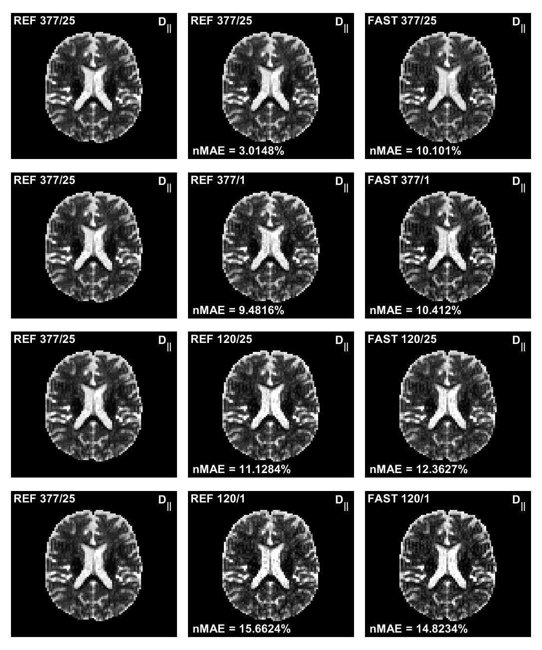
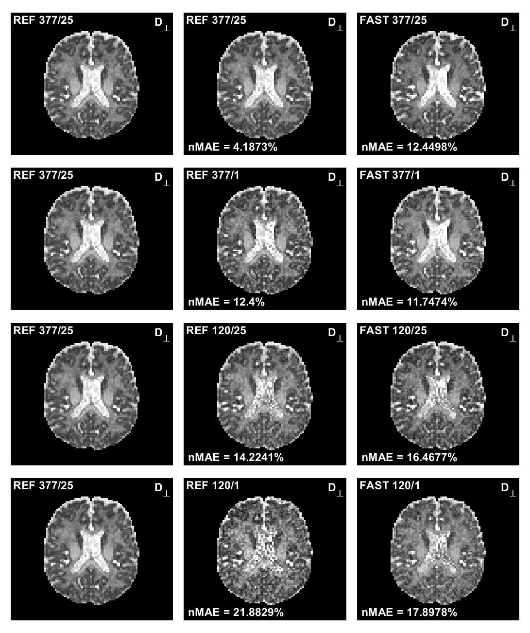
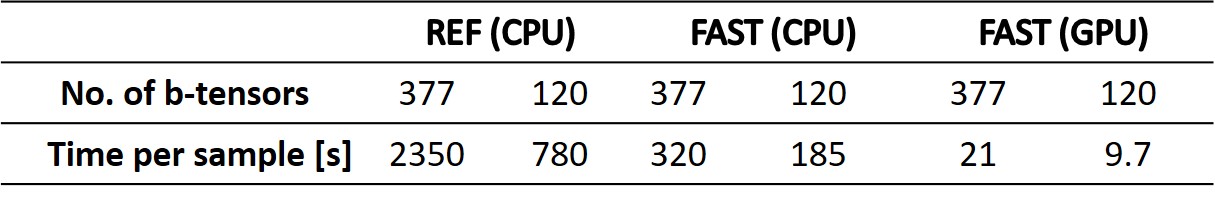
Figure 1 and 2 shows the estimated mean axial and radial diffusivities using both the REF method and the FAST method. As can be seen from the figures, the parameter maps are very similar although not identical. Figure 3 present a summary of the computational times required for a voxel-wise analysis of a 3D volume with 73550 pixels.

Discussion

The goal of this work was to find a fast algorithm for quantitative parameter distribution estimation. This was achieved by a new more precise formulation, suited for GPU implementation, of the underlying mathematical problem. A resulting speed-up factor of up to 7.3 and 242 was observed using CPU and GPU, respectively.
A few observations can be made from Figure 1 and 2:

• Using the FAST method produces less noisy maps compared to the REF method when a single average is used. However, the results does not improve much with many averages as is the case for the REF method.
• The maps from the two different method are very similar, but not identical.

Likely, the difference in the results from the FAST and the REF methods are due to the form of the data consistency constraint. By formulating this as inequality tailored to the noise level there will be some denoising occurring which can affect the final parameter maps. That there is little improvement using many averages for the FAST method is not surprising since it uses a gradient descent method to find an optimum instead of producing Monte-Carlo samples. This also means that a single sample may be enough, which further drastically reduces the computational time needed.

Conclusion

This work shows that it is possible to reduce the time needed to estimate diffusion tensor distributions from possibly several hours to much more clinically useful times in the order of a few seconds to a few minutes.

Acknowledgements

This research was funded by grants from The Swedish Research Council (Grant No. 2019-0432)