2452
A unified framework for estimating diffusion kurtosis tensors with multiple prior information
Li Guo1,2,3, Lyu Jian2,3, Yingjie Mei4, Mingyong Gao1, Yanqiu Feng2,3, and Xinyuan Zhang2,3,5
1Department of MRI, The First People’s Hospital of Foshan (Affiliated Foshan Hospital of Sun Yat-sen University), Foshan, China, 2School of Biomedical Engineering, Southern Medical University, Guangzhou, China, 3Guangdong Provincial Key Laboratory of Medical Image Processing, Southern Medical University, Guangzhou, China, 4Philips Healthcare, Guangzhou, China, 5Guangdong-Hong Kong-Macao Greater Bay Area Center for Brain Science and Brain-Inspired Intelligence, Guangzhou, China
1Department of MRI, The First People’s Hospital of Foshan (Affiliated Foshan Hospital of Sun Yat-sen University), Foshan, China, 2School of Biomedical Engineering, Southern Medical University, Guangzhou, China, 3Guangdong Provincial Key Laboratory of Medical Image Processing, Southern Medical University, Guangzhou, China, 4Philips Healthcare, Guangzhou, China, 5Guangdong-Hong Kong-Macao Greater Bay Area Center for Brain Science and Brain-Inspired Intelligence, Guangzhou, China
Synopsis
Accurate tensor estimation for DKI is usually challenged by noise. The noncentral Chi distribution noise would introduce bias in the estimated DKI tensors. Although several noise-corrected models are statistically unbiased, the DKI tensors generated by these estimators have large variances. In addition, severe noise easily causes the estimated kurtosis values outside a physically acceptable range. The goal of this work is to propose a unified framework that integrates multiple prior information including nonlocal structural self-similarity (NSS), local spatial smoothness (LSS), physical relevance (PR) of DKI model, and noise characteristic of magnitude diffusion images for improved DKI tensor estimation.
Purpose
To propose a unified framework that integrates multiple prior information including nonlocal structural self-similarity (NSS), local spatial smoothness (LSS), physical relevance (PR) of DKI model, and noise characteristic of magnitude diffusion MRI (dMRI) images for improved DKI tensor estimation.Methods
The diffusion tensor (DT) and kurtosis tensor (KT) of all pixels across the image (namely DT and KT fields) are simultaneously estimated by our unified estimation framework. Suppose the size of a 2D image is M×N, the unified estimation framework for DT field Df$$$\in$$$RM×N×3×3 and KT field Wf$$$\in$$$RM×N×3×3×3×3 can be formulated as:$$\min_{ {\bf \theta} }F({\bf \theta})=\min_{ {\bf \theta} }\{\sum_{ x_{i}\in Ω}\sum_{ x_{j}\in V_{i}}w(x_{i},x_{j})\sum_{n=1}^{N_{DWI}}\|S_{m}(b_{n};{g_{n}};x_{j})-f(b_{n};{g_{n}};{\bf \theta}(x_{i}))||_{2}^{2}+\lambda\sum_{q=1}^{Q}TV({\bf \theta}_{q})+R({\bf \theta}_{D_{f}},{\bf \theta}_{W_{f}})\}$$(1)Here, the first term is a weighted nonlinear least squares term which incorporates the nonlocal structural self-similarity (NSS) prior information to reduce the noise effect on the model fitting. θ$$$\in$$$RM×N×Q denotes all the parameter maps where Q is the total number of DKI model parameters for each pixel. Sm is the measured signal with the diffusion weighting strength bn along the gradient direction gn, f(⁕) the first-moment noise-corrected model (M1NCM) as a function of θ and can be formulated as:$$f({\bf \theta})=\sigma\sqrt{\frac{\pi}{2}}\frac{(2C-1)!!}{2^{C-1}(C-1)!!}F_{1}^{1}(-0.5;C;(\frac{S(b;g;{\bf \theta})}{\sqrt{2}\sigma})^{2})$$(2)
where σ the standard deviation (SD) of complex Gaussian noise, C the number of coils, !! the double factorial, $$$F_{1}^{1}$$$the confluent hypergeometric function, S the underlying noise-free signal. w(xi, xj) is the weight that controls the contribution of neighboring pixel xj within search window Vi to the tensor estimation of target pixel xi within image domain Ω and is defined as:$$w(x_{i},x_{j})=\frac{1}{Z(x_{i})}exp(-\frac{_{G_{a}\|P_{i}-P_{j}||_{2}^{2}}}{h^{2}}),\forall x_{j}\in V_{i} and x_{j}\neq x_{i}$$(3)
where Z(xi) is the normalized constant, Ga a normalized Gaussian kernel (the SD of a), h controls the degree of smoothing and determined as h = βσ, where β is a scalar. Pi and Pj denote 3D patch of p×p×NDWI, where p is the patch size in the spatial domain, and the patch size along the diffusion dimension is set to the total number of non-DW and DW images (NDWI).
The second term is a total variation (TV) regularization term which constraints the local spatial smoothness (LSS) on each parameter map θq$$$\in$$$RM×N.
The third term ensures that the DKI model is physically relevant1,2. For each diffusion encoding direction g, we use the following function to construct the R(θDf, θWf):$$R({\bf \theta}_{D_{f}},{\bf \theta}_{W_{f}})=\sum_{ x_{i}\in Ω}\sum_{n=1}^{N_{DWI}}(exp(\frac{{K_{f}(g_{n},x_{i})-3/b_{max}/}D_{f}(g_{n},x_{i})}{c_{1}})+exp(\frac{{K_{f}(g_{n},x_{i})}}{c_{2}}))$$(4)
Here, c1 and c2 are small values to ensure R(θDf, θWf) approaches infinity (or a big number) when the physical relevance is not satisfied. We solved the unconstrained nonlinear optimization problem (Eq. (1)) by using the limited-memory BFGS Quasi-Newton method (L-BFGS).
To quantitatively evaluate the performance of the proposed M1NCM-NSS-LSS-PR algorithm, simulations were performed based on one subject (“100307”) from HCP diffusion data3. First, the reference DKI tensors were estimated using constrained weighted least square estimator4 after preprocessing of denoising and bias correction. Second, the estimated DKI tensors were used to simulate the reference data with one non-DW image and 45 b = 1000 and 45 b = 2000 s/mm2 DW images. Third, the reference serial images were used to generate noncentral Chi (C = 8) distributed serial images with stationary noise levels of 0.02, 0.03, 0.04, 0.05, 0.06, 0.07, 0.08, 0.09 and unstationary noise levels of 0.02 and 0.03. A modulation map with factors 1-3 was multiplied with the unstationary noise level to generate the spatially unstationary noise. The Gaussian noise can be computed in advance by using background area for stationary noise case and be treated as an unknown parameter for unstationary noise case.
To validate the effect of introducing different prior information on the estimation of DKI parameters, we compared the following M1NCM-based methods: 1) M1NCM; 2) M1NCM-NSS; 3) M1NCM-LSS; 4) M1NCM-NSS-LSS; 5) M1NCM-NSS-LSS-PR. We also compared the proposed M1NCM-NSS-LSS-PR algorithm with two widely used methods: nonlinear least squares (NLS) and constrained weighted linear least squares (CWLLS)4. For the sake of fairness, we adopted an unbiased vector nonlocal means (UVNLM) filter5 to denoise and correct the noise bias prior to the NLS or CWLLS estimation (referred as UVNLM-NLS and UVNLM-CWLLS, respectively).
Results
Fig. 1 presents the RMSEs of FA, MD, MK maps estimated by the different algorithms, using the simulated data with stationary noise levels of 0.02-0.09. Table 1 shows the RMSE values of the FA, MD, MK maps as well as the noise maps estimated by the proposed M1NCM-based algorithms, using the simulated data with unstationary noise levels of 0.02 and 0.03. In terms of RMSE for each parameter map, M1NCM-NSS-LSS and M1NCM-NSS-LSS-PR outperformed other compared algorithms at all the noise levels. In Figs. 2 and 3, a visual comparison of the estimated FA, MD, MK maps and their corresponding error maps is presented. It can be seen that the parameter maps from the proposed M1NCM-NSS-LSS or M1NCM-NSS-LSS-PR methods had the minimum errors and were visually closest to the reference parameter maps among all compared methods.Discussion and conclusion
The proposed M1NCM-NSS-LSS-PR outperformed the compared methods on the simulated data with both the spatially stationary and unstationary noise distributions. The proposed method can be easily extended to a 3D version for the volume diffusion data, which will further improve the accuracy of DKI tensor estimation.Acknowledgements
This study was funded by China Postdoctoral Science Foundation (NO.2020M672526), Guangdong Basic and Applied Basic Research Foundation (NO.2019A1515110976), National Natural Science Foundation of China (NO.61971214, 81601564), Natural Science Foundation of Guangdong Province (NO.2019A1515011513), Guangdong-Hong Kong-Macao Greater Bay Area Center for Brain Science and Brain-Inspired Intelligence Fund (NO.2019022).References
[1] Veraart, J., et al. “Constrained maximum likelihood estimation of the diffusion kurtosis tensor using a rician noise model”. Magn Reson Med 66, 678-686. (2011). [2] Tabesh, A., et al. “Estimation of tensors and tensor-derived measures in diffusional kurtosis imaging”. Magn Reson Med 65, 823-836. (2011). [3] https://www.humanconnectome.org/ [4] Veraart, J., et al. “Weighted linear least squares estimation of diffusion mri parameters: Strengths, limitations, and pitfalls”. Neuroimage 81, 335-346. (2013). [5] Zhou, M.X., et al. “Evaluation of non-local means based denoising filters for diffusion kurtosis imaging using a new phantom”. PLoS One 10, e0116986. (2015).Figures
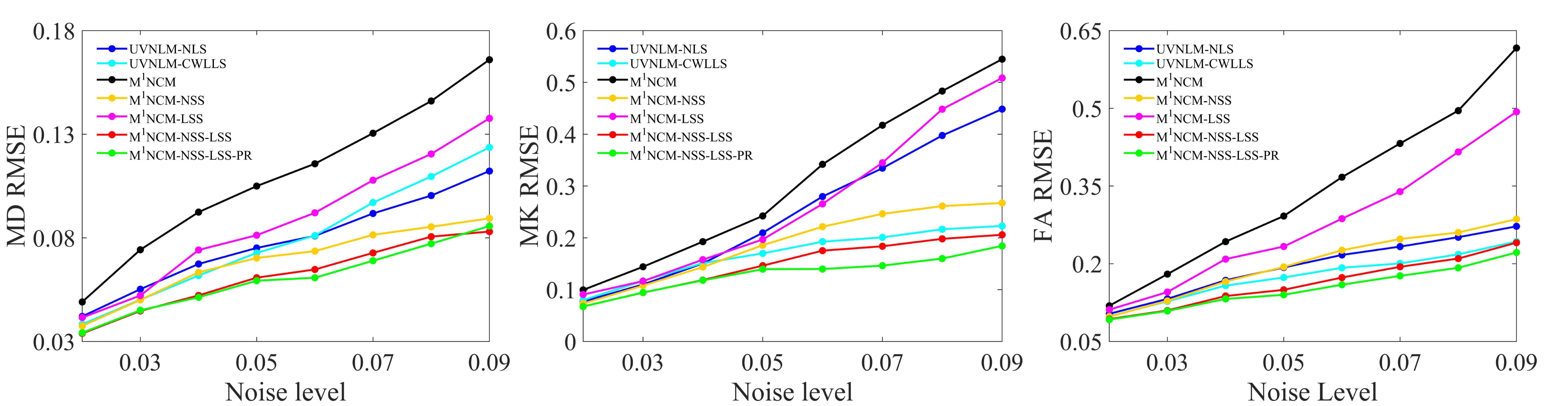
Figure 1. RMSE comparisons of FA,
MD, MK maps estimated with the UVNLM-NLS, UVNLM-CWLLS, M1NCM, M1NCM-NSS,
M1NCM-LSS, M1NCM-NSS-LSS, and M1NCM-NSS-LSS-PR
algorithms, using the simulated datasets with stationary and fixed noise levels
of 0.02-0.09.
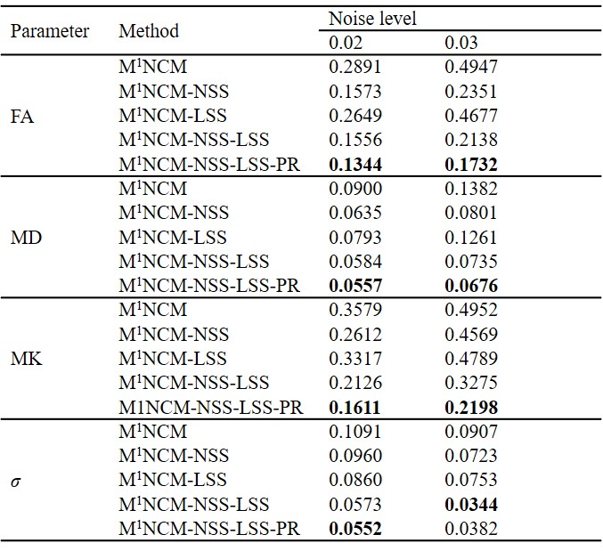
Table 1. RMSE values of FA, MD, MK maps as well as noise SD
maps (σ) estimated with the proposed
M1NCM-based algorithms (M1NCM, M1NCM-NSS, M1NCM-LSS,
M1NCM-NSS-LSS, and M1NCM-NSS-LSS-PR), using the simulated
datasets with unstationary and unfixed noise levels of 0.02 and 0.03. Best
results are
highlighted in bold.
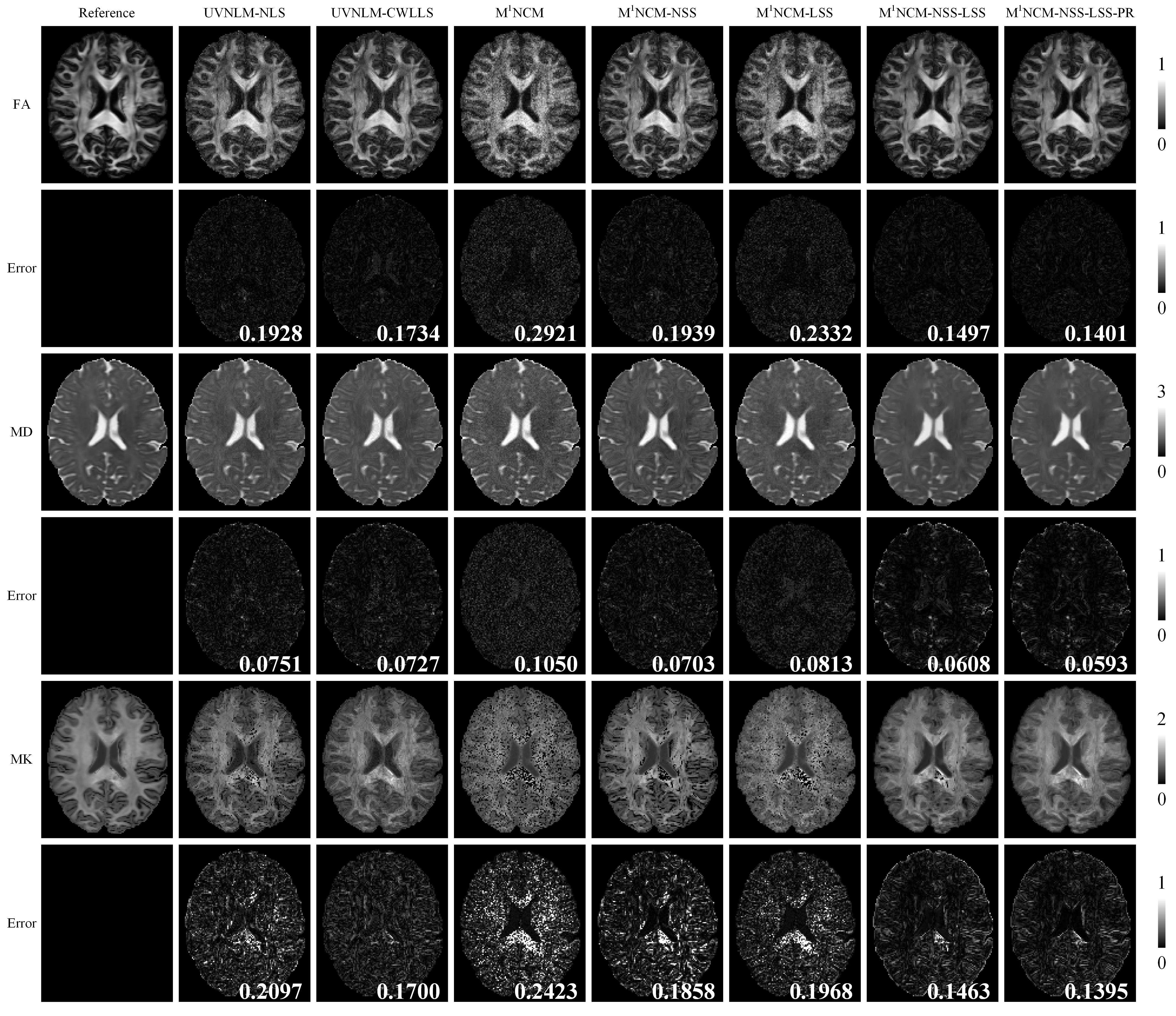
Figure 2. FA, MD, MK maps and their corresponding error maps
of the UVNLM-NLS, UVNLM-CWLLS, M1NCM, M1NCM-NSS, M1NCM-LSS,
M1NCM-NSS-LSS, and M1NCM-NSS-LSS-PR, using the simulated data
with stationary noise level of 0.05. The error maps show the absolute
difference between the reference parameters and the estimated parameters. The
RMSE of each parameter map is shown in the right bottom of its error map. The
unit of the MD is ×10-3 mm2/s.
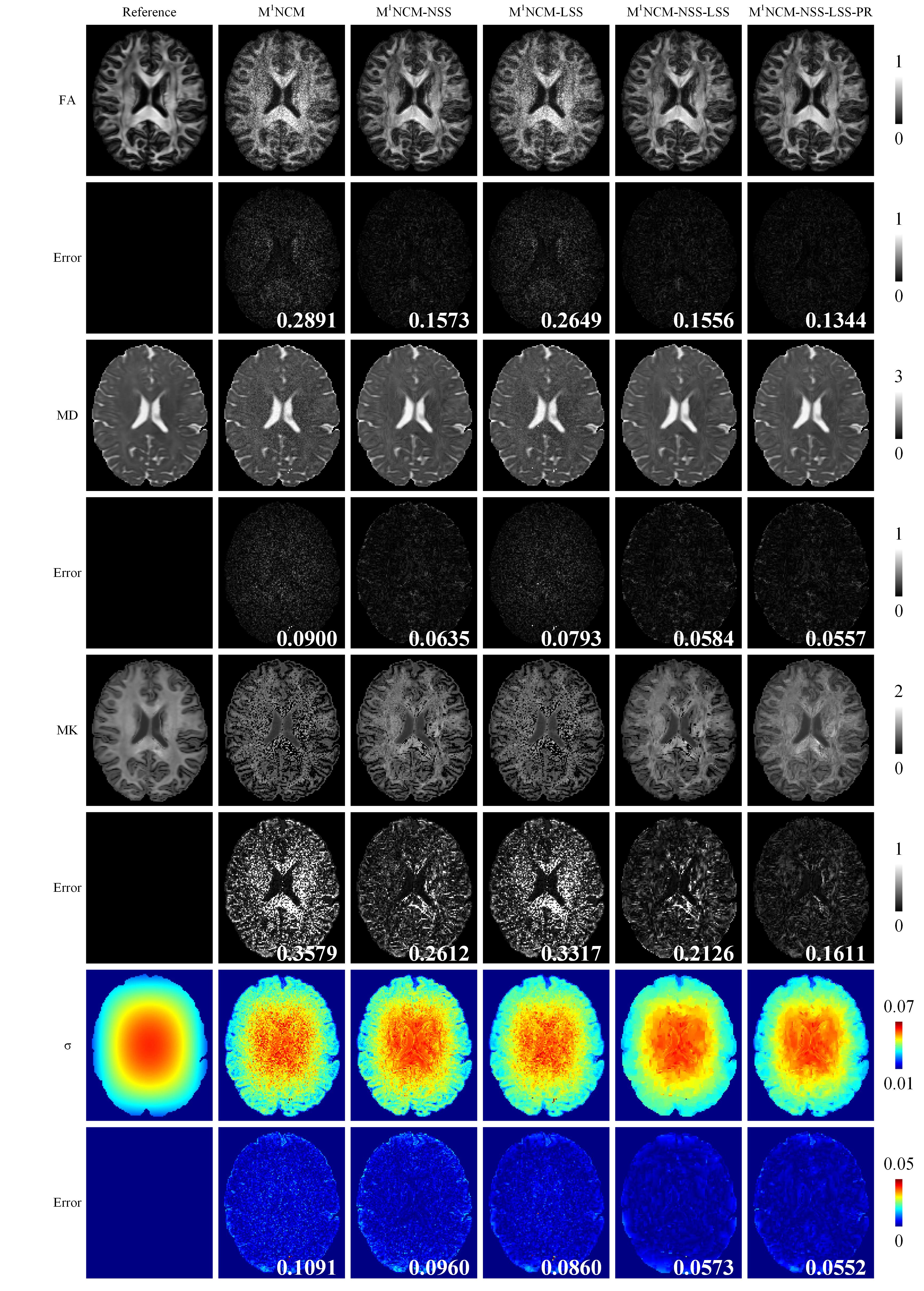
Figure 3. FA, MD, MK, noise SD (σ) maps and
their corresponding error maps of the M1NCM-based methods, using the
simulated data with unstationary noise level of 0.02. The error maps show the
absolute difference between the reference parameters and the estimated
parameters. The RMSE of each parameter map is shown in the right bottom of its
error map. The unit of the MD is ×10-3 mm2/s.