Introduction

Convolutional networks are very successful in medical imaging because they are translation-equivariant, i.e. they detect features well, regardless of their translation (location). Recently, neural networks that are equivariant under 3D rotations and translations (i.e. the group $$$\mathrm{SE}(3)$$$) were proposed and proved even more successful^1,2. Learning the many possible orientations of a feature (e.g. a neural fiber) is more complicated than generalizing automatically to all orientations via $$$\mathrm{SE}(3)$$$-equivariance. In diffusion MRI (dMRI), deep learning is highly beneficial³ and $$$\mathrm{SE}(3)$$$-equivariance is appropriate because neural fibers can have a large variety of orientations. So far, $$$\mathrm{SE}(3)$$$-equivariant networks have been proposed only for 3D data. Here we propose $$$\mathrm{SE}(3)$$$-equivariant networks for 6D dMRI data and demonstrate their benefits.

Methods

An $$$\mathrm{SE}(3)$$$-equivariant network layer was proposed for 3D point clouds¹ and 3D images². Both approaches use $$$\mathrm{SE(3)}$$$-equivariant filters built as weighted sums from pre-defined basis filters that use spherical harmonics as their angular part, and a radial basis. Feature maps are so-called spherical-tensor fields of possibly different orders for each channel^1,2. These spherical tensors are combined with the filter using Clebsch–Gordan coefficients.

A roto-translation of an object in the scanner causes a roto-translation of the image in position space ($$$p$$$-space) and rotation in $$$q$$$-space. We propose a network layer that respects this dMRI-inherent equivariance. We generalize prior work^1,2 from 3D data to the 6D space of dMRI scans.

As $$$q$$$-space is not translated, we multiply two radial bases: on the input and output $$$q$$$-vector lengths, respectively. For the angular part, we use the spherical harmonics twice: once applied to $$$p$$$- and once to $$$q$$$-space coordinate offsets. Both are combined into the angular part of the basis filters using Clebsch–Gordan coefficients. This leads to the following definition of our proposed layer $$$\mathcal{L}$$$:
$$\mathcal{L}_{m_{\mathrm{out}}}^{(c_{\mathrm{out}})}[\mathbf{I}](\mathbf{p}_{\mathrm{out}},\mathbf{q}_{\mathrm{out}})=\sum_{c_{\mathrm{in}},l_{\mathrm{filter}},l_p,l_q,k_1,k_2,k_3}W_{c_{\mathrm{in}},c_{\mathrm{out}},k_1,k_2,k_3}^{(l_{\mathrm{filter}},l_p,l_q)} \sum_{\substack{m_{\mathrm{filter}}\in\{-l_{\mathrm{filter}},\dots,l_{\mathrm{filter}}\},\\ m_{\mathrm{in}}\in\{-l_{\mathrm{in}},\dots,l_{\mathrm{in}}\}}}C_{(l_{\mathrm{filter}}, m_{\mathrm{filter}})(l_{\mathrm{in}},m_{\mathrm{in}})}^{(l_{\mathrm{out}},m_{\mathrm{out}})}\\ \qquad\times\sum_{\substack{\mathbf{p}_{\mathrm{in}}\in\mathbb{R}^3,\\ \mathbf{q}_{\mathrm{in}}\in\mathbb{R}^3}} \varphi_1^{(k_1)}(\left\lVert\mathbf{p}_{\mathrm{out}}-\mathbf{p}_{\mathrm{in}}\right\rVert_2)\varphi_2^{(k_2)}(\left\lVert\mathbf{q}_{\mathrm{out}}\right\rVert_2)\varphi_3^{(k_3)}(\left\lVert\mathbf{q}_{\mathrm{in}}\right\rVert_2)\\ \qquad\times\sum_{\substack{m_p\in\{-l_p,\dots,l_p\},\\ m_q\in\{-l_q,\dots,l_q\}}}C_{(l_p, m_p)(l_q,m_q)}^{(l_{\mathrm{filter}},m_{\mathrm{filter}})}Y_{m_p}^{(l_p)}\left(\frac{\mathbf{p}_{\mathrm{out}}-\mathbf{p}_{\mathrm{in}}}{\left\lVert\mathbf{p}_{\mathrm{out}}-\mathbf{p}_{\mathrm{in}}\right\rVert_2}\right)Y_{m_q}^{(l_q)}\left(\frac{\mathbf{q}_{\mathrm{out}}-\mathbf{q}_{\mathrm{in}}}{\left\lVert\mathbf{q}_{\mathrm{out}}-\mathbf{q}_{\mathrm{in}}\right\rVert_2}\right)I_{m_{\mathrm{in}}}^{(c_{\mathrm{in}})}(\mathbf{p}_{\mathrm{in}},\mathbf{q}_{\mathrm{in}}),$$
where $$$\mathbf{I}$$$ denotes the input feature map, $$$\mathbf{p}_{\mathrm{out}}$$$ and $$$\mathbf{q}_{\mathrm{out}}$$$ are $$$p$$$- and $$$q$$$-space coordinates in the output and $$$\mathbf{p}_{\mathrm{in}}$$$, $$$\mathbf{q}_{\mathrm{in}}$$$ in the input feature map, $$$c_{\mathrm{out}}$$$ is the index of one of the output channels, $$$l_{\mathrm{out}}$$$ is shorthand for $$$l_{\mathrm{out}}(c_{\mathrm{out}})$$$, i.e. the order of the output channel $$$c_{\mathrm{out}}$$$, $$$m_{\mathrm{out}}$$$ indices the components of the output tensor of channel $$$c_{\mathrm{out}}$$$, with $$$-l_{\mathrm{out}}\le m_{\mathrm{out}}\le l_{\mathrm{out}}$$$, the index $$$c_{\mathrm{in}}$$$ goes over all input channels, $$$l_{\mathrm{in}}$$$ is shorthand for $$$l_{\mathrm{in}}(c_{\mathrm{in}})$$$, i.e. the order of the input channel $$$c_{\mathrm{in}}$$$, with $$$-l_{\mathrm{in}}\le m_{\mathrm{in}}\le l_{\mathrm{in}}$$$, $$$l_{\mathrm{filter}}$$$ is the filter order (frequency index) used to index the angular filter basis, with $$$|l_{\mathrm{out}}-l_{\mathrm{in}}|\le l_{\mathrm{filter}}\le(l_{\mathrm{out}}+l_{\mathrm{in}})$$$, $$$l_p$$$ and $$$l_q$$$ are the orders of the p- and q-space parts of the filter, with $$$|l_p-l_q|\le l_{\mathrm{filter}}\le (l_p+l_q)$$$, and $$$|l_{\mathrm{filter}}-l_p|\le 1$$$, $$$k_1, k_2, k_3$$$ are indices of the radial bases for $$$p$$$-space coordinate offsets and $$$q$$$-space output and input coordinates, $$$\mathbf{W}$$$ are learned weights, $$$\mathbf{C}$$$ are the (real) Clebsch–Gordan coefficients, $$$\varphi_1^{(k_1)}:\mathbb{R}_{\ge 0}\rightarrow\mathbb{R}$$$, $$$\varphi_2^{(k_2)}:\mathbb{R}_{\ge 0}\rightarrow\mathbb{R}$$$, $$$\varphi_3^{(k_3)}:\mathbb{R}_{\ge 0}\rightarrow\mathbb{R}$$$ are sets of radial bases, $$$\mathbf{Y}$$$ are the (real) spherical harmonics.

The derivation and proof of equivariance are a generalization of prior work^1,2 to 6D dMRI data.

Note that the only learnable parameters are $$$\mathbf{W}$$$ and optional parameters in $$$\varphi_1^{(k_1)}$$$, $$$\varphi_2^{(k_2)}$$$, and $$$\varphi_3^{(k_3)}$$$. The proposed layer is not the only option how a generalization of the equivariant 3D layer to dMRI is possible, we also investigated applying the spherical harmonics only once to the difference of coordinate offsets from $$$p$$$- and $$$q$$$-space but found it to be less effective.

The effectivity of the proposed layer is studied by doing segmentation of multiple sclerosis (MS) lesions using a dataset⁴ containing dMRI brain scans with ground-truth annotations of MS lesions. Our architecture uses five of the proposed equivariant layers. Various hyperparameters yielded similar results. Each of the layers is followed by a gated nonlinearity¹ and swish⁵ for scalar channels, except for the last layer, which uses sigmoid.

Results & Discussion

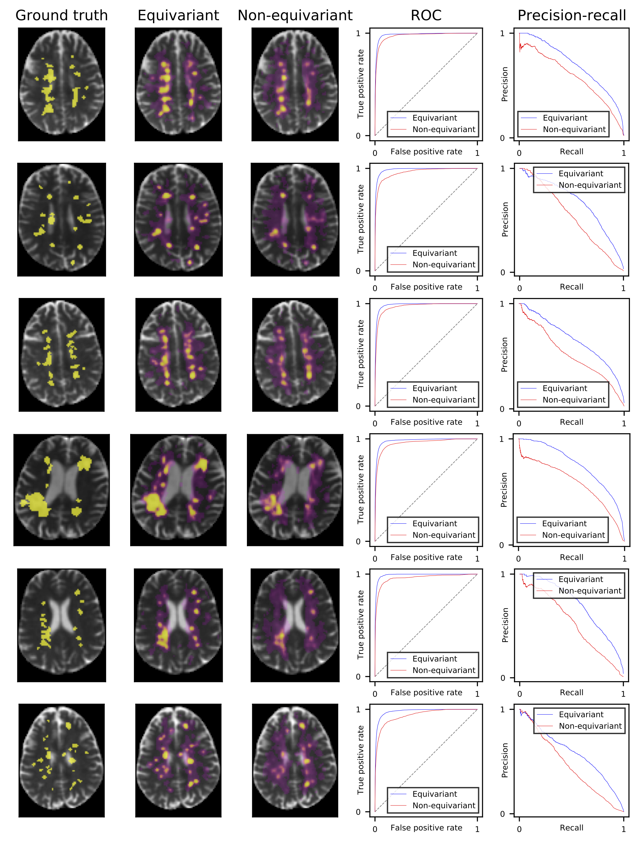
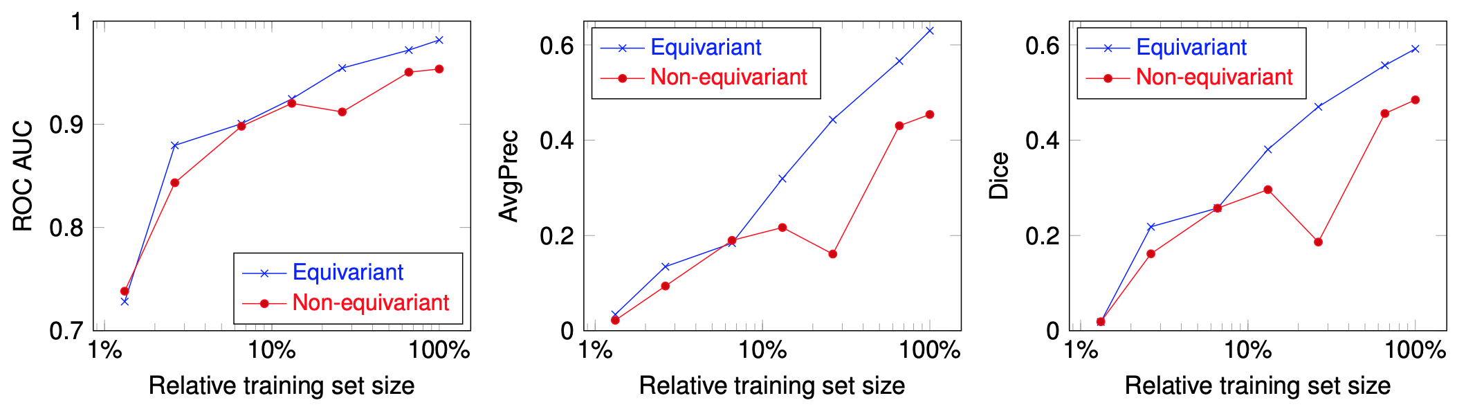
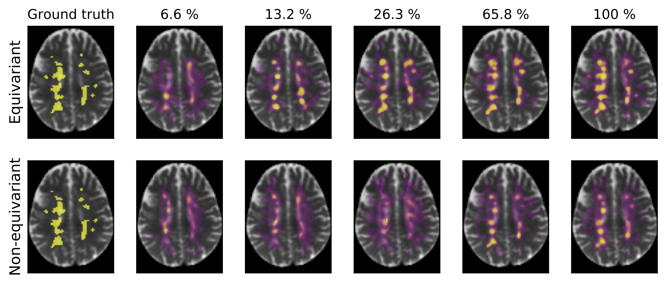
Fig. 1 shows the segmentation of six scans from the validation set (not used for training) with ground truth, predictions from our model, and a non-rotation-equivariant reference model that uses 3D convolutional layers, and shows their receiver operating characteristic (ROC) and precision-recall curves. Our model achieves 0.982 area under the ROC curve (AUC), 0.630 average precision (AvgPrec), and 0.592 Dice score. Figs. 2-3 show how the models are affected when the training dataset size is reduced.

While already the non-rotation-equivariant model roughly predicts the ground truth, our model predicts it more accurately. It can especially be seen that while our model predicts the MS lesions very confidently and reports very small values outside the areas around the lesions, the non-rotation-equivariant model is very uncertain at many positions. Our model outperforms the non-rotation-equivariant model by 3% ROC AUC, 39% AvgPrec, and 22% Dice score. Also, our model requires four times fewer training samples than the non-rotation-equivariant model to achieve comparable quality.

Conclusions

Our results show that the proposed layer can increase the performance through better generalization and decrease the required number of training samples on dMRI datasets. The equivariance of the layer allows the use of many parameters that can effectively capture the essence of the dataset so that the model does not underfit while still restricting it so that overfitting is effectively reduced without using additional regularization. Thus, the method likely improves results on other dMRI datasets.

Acknowledgements

This work was supported by the Munich Center for Machine Learning (Grant No. 01IS18036B) and the BMBF project MLwin.