2416
Quantification of Unsuppressed Water Spectrum using Autoencoder with Feature Fusion
Marcia Sahaya Louis1,2, Eduardo Coello2, Huijun Liao2, Ajay Joshi1, and Alexander P Lin2
1Boston University, Boston, MA, United States, 2Brigham and Women's hospital, Boston, MA, United States
1Boston University, Boston, MA, United States, 2Brigham and Women's hospital, Boston, MA, United States
Synopsis
Recent years have witnessed novel applications of machine learning in radiology. Developing robust machine learning based methods for removing spectral artifacts and reconstructing the intact metabolite spectrum is an open challenge in MR spectroscopy (MRS). We had shown autoencoder models reconstruct metabolite spectrum from unsuppressed water spectrum for short TE with relatively high SNR. In this work we presents an autoencoder model with feature fusion method to extract the shallow and deep features from a water unsuppressed 1H MR spectrum. The model learns to map the extracted feature to a latent code and reconstruct the intact metabolite spectrum
Introduction
MR Spectroscopy (MRS) non-invasively monitors metabolites to diagnose or monitor brain tumors1. Specifically, the 97ms TE MRS technique is useful for diagnosing low-grade gliomas by detecting 2-hydroxyglutarate (2HG), a biomarker for isocitrate dehydrogenase mutations2. Some disadvantages of MRS of the brain include the presence of water resonance3, which leads to failure to detect low abundance metabolites. Also, incomplete suppression of the water signal adds biases in the current models used for MRS quantification4–6. Therefore, models must remove water while preserving both low and high concentration metabolites. We had shown previously that the autoencoder model could reconstruct metabolite spectra from unsuppressed water acquisitions7. The data used in the previous work was acquired using 30 ms TE with relatively high SNR and a homogeneous cohort of subjects. However, the tumor spectrum is highly variable, and the detection of 2HG is more challenging. The goal of this work is to remove water resonance from 97 ms TE spectra and to use feature fusion to preserve shallow and deep features to measure 2HG, which has very low concentrationsMethods
Autoencoder Model: The architecture of the autoencoder model in Figure 1 has two sub-networks: encoder and decoder. The autoencoder model takes an unsuppressed water spectrum as the network input and reconstructs the metabolite spectrum as the network output. The encoder network is a deep convolutional neural network. The feature extracted by deep convolutional layers gradually saturates, leading to loss of low concentration metabolite information. On the other hand, shallow features would only include global information with minimal information about high concentration metabolites. Therefore, the encoder network combines features from different layers of the network and maps it to a lower-dimensional manifold (z). The decoder network reconstructs the metabolite spectrum using the z. With this approach, the model learns a vector field for mapping the input water signal to z and is trained to remove the water resonance while preserving metabolite resonances effectively.Data: We used single-voxel spectroscopy acquired in IDH+ brain tumors (n=355; PRESS TE/TR: 97/2000ms, 128 averages, 8 cc volume) to train and evaluate the autoencoder model. We applied frequency, phase, and eddy current correction using OpenMRSLab tools8. We created a semi-synthetic dataset by linearly combining in-vivo spectra to a single water signal to choose the hyper-parameters of the autoencoder model. The dataset was randomly divided into a 67% training set and a 33% test set. We performed data augmentation by combining two different spectra iteratively and increased the training size to n=12000. The model was trained using TensorFlow9 with Adamoptimizer10 as a method for stochastic optimization. We used mean squared error to estimate the reconstruction loss of the model. After the training process, the model was evaluated on the test set. Figure 2 shows the mean and standard deviation of the water suppressed spectra, and autoencoder predicted spectra. The spectra were quantified using LC-model5 to evaluate the autoencoder predicted spectra quantification capacity. The hyper-parameters of the model were selected based on the quantification capacity of the reconstructed spectra. The autoencoder model with the chosen hyper-parameters was trained and evaluated using the complete in-vivo dataset with a 67%/33% training-test set split. The model was trained on the training set with data augmentation (n=12000) and evaluated on the test set (n=120). The quantification capacity of the reconstructed spectrum was evaluated using LC-Model.
Results and Discussion
The mean and standard deviation of water suppressed spectra and autoencoder reconstructed spectra are shown in Figure 2. We can observe from Figure 2A and B that the model could effectively reconstruct resonance of low and high concentration metabolites. The reconstructed spectrum was also able to preserve the metabolite spectrum's diagnostic capability compared to the previous autoencoder model7, which is shown in Figure 3. We evaluated the reconstructed spectrum's quantification capability using LC-Model and compared it with the corresponding water suppressed spectrum. We computed the Pearson-R2 value between the two spectrums for total N-acetyl-aspartate (tNAA), total choline (tCho), creatine (tCr), glutamate and glutamine (Glx), lactate (Lac), glutathione (GSH), myo-inositol (mI) and 2-hydroxyglutarate (2HG). Figure 4 summarizes the search of hyper-parameters of the autoencoder model. The autoencoder model with a kernel size of 9, a model with 16 layers, and a latent vector dimension of 128 was selected based on the R2 value of eight metabolites of interest. The best model was trained and evaluated on the in-vivo dataset. We also quantified the water unsuppressed spectrum using LC-Model to estimate the baseline performance (Figure 4C). The scatter-plot in Figure 5 shows the correlation between the water suppressed spectrum and the reconstructed spectrum for the in-vivo test dataset.Conclusion
This work presented a machine learning approach for water removal while preserving the diagnostic value of the metabolite spectrum. The feature fusion method used shallow and deep features of the water unsuppressed spectrum to reconstruct the metabolite spectrum. Therefore, allows estimating low and high concentration metabolites without water suppression. Spectra acquired without water suppression has the advantage of providing an internal reference for quantification. It is particularly advantageous in MRSI methods11 by eliminating a second time-consuming reference scan.Acknowledgements
This work was supported by the Innovation Discovery Grant award.References
- Lin, A. et al. Efficacy of proton magnetic resonance spectroscopy in neurological diagnosis and neurotherapeutic decision making. NeuroRx 2.2, 197–214 (2005)
- Zhou, M.et al. Diagnostic accuracy of 2-hydroxyglutarate magnetic resonance spectroscopy in newly diagnosed brain mass and suspected recurrent gliomas.Neuro-oncology20, 1262–1271 (2018)
- Govindaraju, V. et al. Proton NMR chemical shifts and coupling constants for brain metabolites. NMR in Biomedicine: An International Journal Devoted to the Development and Application of Magnetic Resonance In Vivo13, 129–153 (2000)
- Wilson, M.et al. A constrained least-squares approach to the automated quantitation of in vivo 1H magnetic resonance spectroscopy data. Magnetic Resonance in Medicine 65, 1–12 (2011)
- Provencher, S. W. Automatic quantitation of localized in vivo 1H spectra with LCModel. NMR in Biomedicine 14, 260–264 (2001)
- Soher, B.et al. Vespa: integrated applications for rf pulse design, spectral simulation and MRS data analysis. InProc Int Soc Magn Reson Med, vol. 19, 1410 (2011)
- Louis, M., Coello, E., Liao, H., Joshi, A. & Lin, A. Quantification of magnetic resonance spectroscopy with unsuppressed water signal(2020)
- Rowland B, I. J. L. A., Mariano LJ. An open-source software repository for magnetic resonance spectroscopy data analysis tools.International Society for Magnetic Resonance in Medicine MR Spectroscopy Workshop(2016)
- Abadi, M.et al. Tensorflow: A system for large-scale machine learning. In12th{USENIX}Symposium on Operating Systems Design and Implementation , 265–283 (2016)
- Kingma, D. P.et al. Auto-encoding variational Bayes. arXiv preprint arXiv:1312.6114 (2013)
- Gasparovic, C.et al. Use of tissue water as a concentration reference for proton spectroscopic imaging. Magnetic Resonance in Medicine 55, 1219–1226 (2006).
Figures
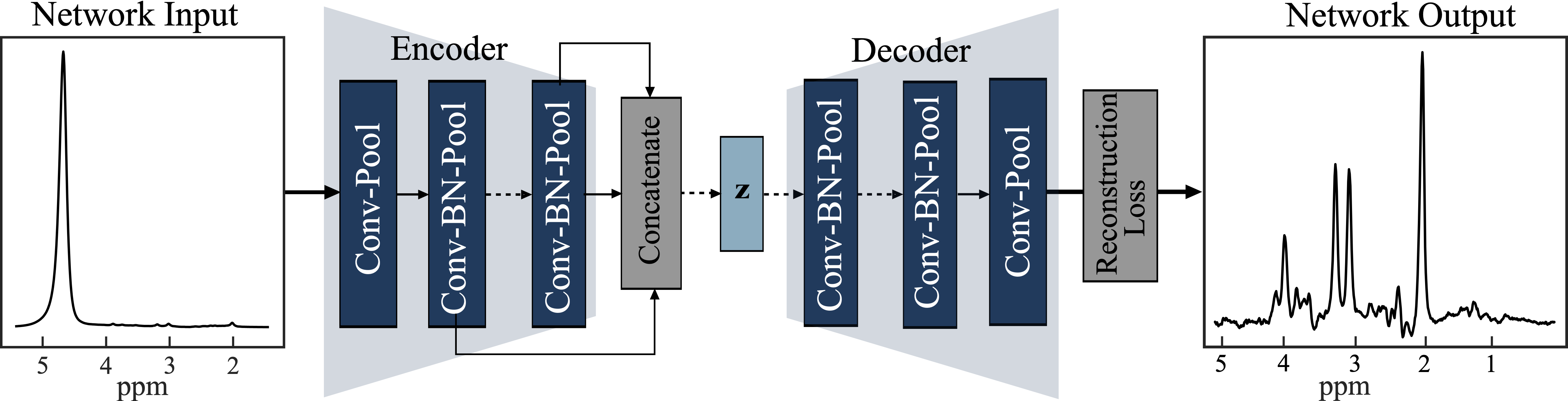
Architecture of Autoencoder with Feature Fusion. The encoder and decoder each have eight convolutional (conv) layers with pooling and batch normalization (BN). Each conv layer had a kernel size of 9 and 16 filters and one fully connected layer with 1000 hidden units. The feature maps of all the layers in the encoder are concatenated using maximum pooling and passed to the latent vector (Z). Z is a fully connected layer with 128 hidden units with a linear activation function. All the layers in the model have a ReLU activation function, except the last layer has a tanh activation function.
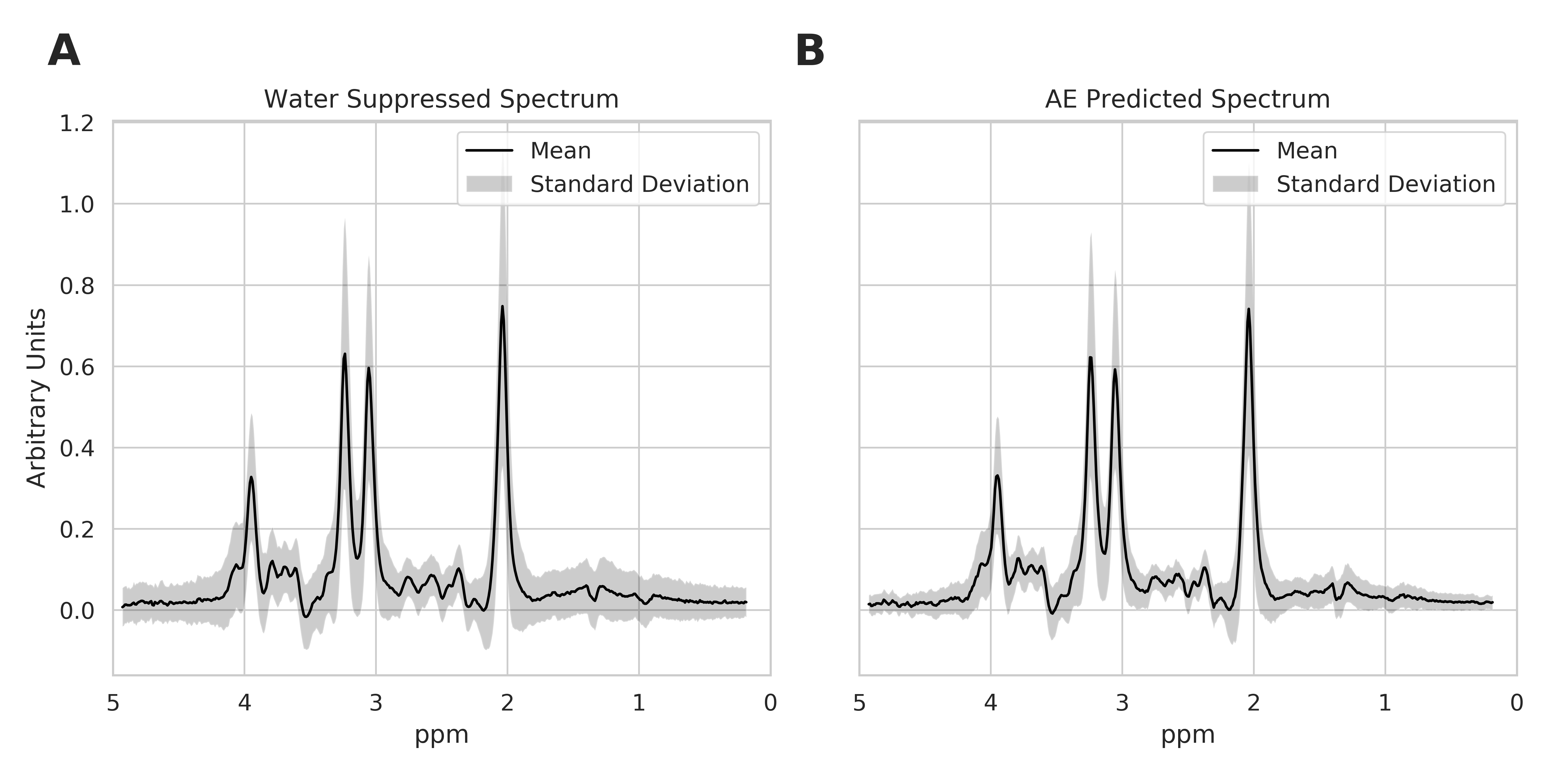
Mean and standard deviation of the Water Suppressed Spectrum and AE predicted spectrum from in-vivo test dataset. The spectra in the dataset were normalized to the height of the peak with maximum intensity. Comparing A and B shows that the autoencoder model is capable of capturing low and high concentration peaks.
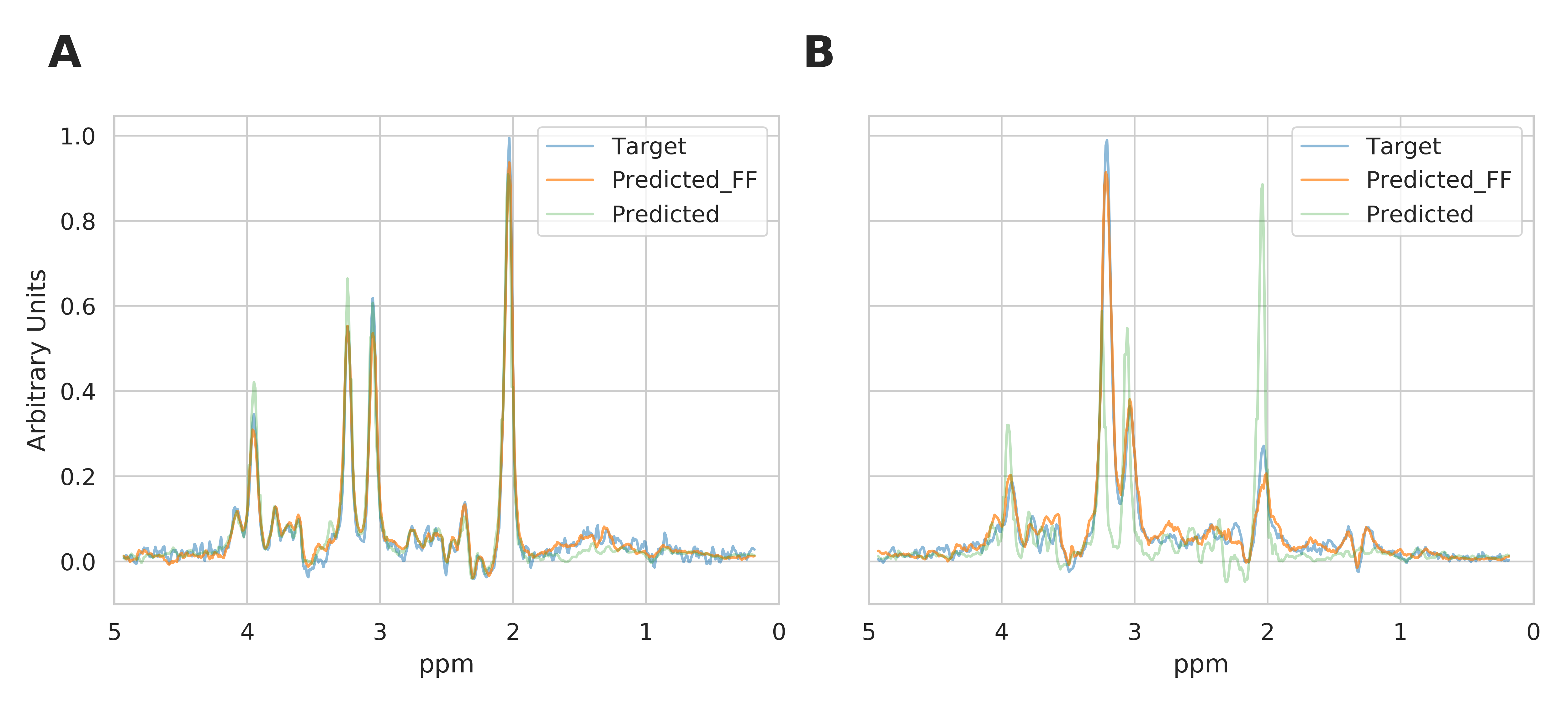
Overlay of water suppressed metabolite spectrum (Target), the corresponding autoencoder predicted metabolite spectrum using feature fusion (Predict_FF) and autoencoder without feature fusion predicted metabolite spectrum (Predict). The Target, Predict_FF and Predict spectrum are very similar to each other for a healthy subject in Figure A. The Target, Predict-FF spectrum are very similar, but the Predict spectrum completely mispredicts the tumor spectrum in Figure B. The autoencoder model with feature fusion is capable of preserving the diagnostic value of the spectrum.
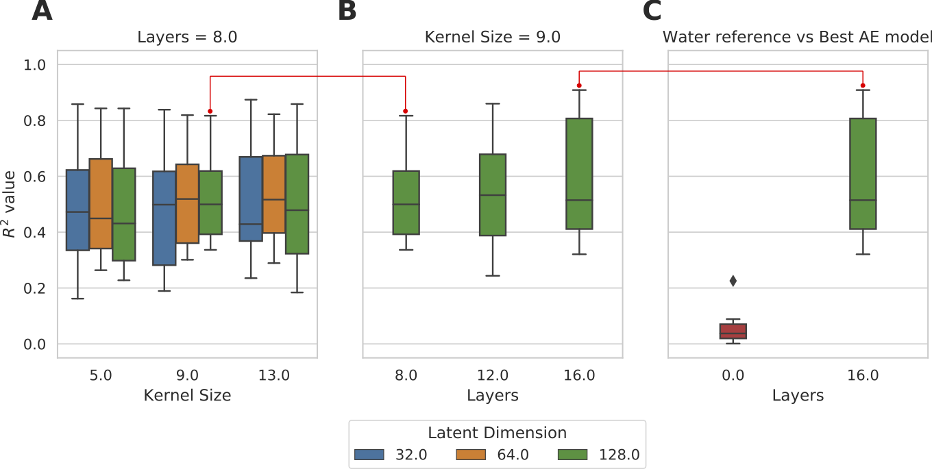
Boxplot of R2 of metabolite concentration
(AE) predicted and water
suppressed spectra for semi-synthetic test dataset. The maximum of boxplot corresponds to tNAA, tCho, tCr, and minimum correspond Glx, Lac, GSH, mI, 2HG. Figure A shows grid-search result for an 8-layer model has a high correlation for Kernel size of 9 and Latent dimension of 128. Figure B shows effect of increasing the number of layers for kernel size of 9 and the best model has kernel size is 9, Latent dimension is 128, and 16 layers. Figure C shows boxplot of R2 of the best model and quantified water spectra for comparison.
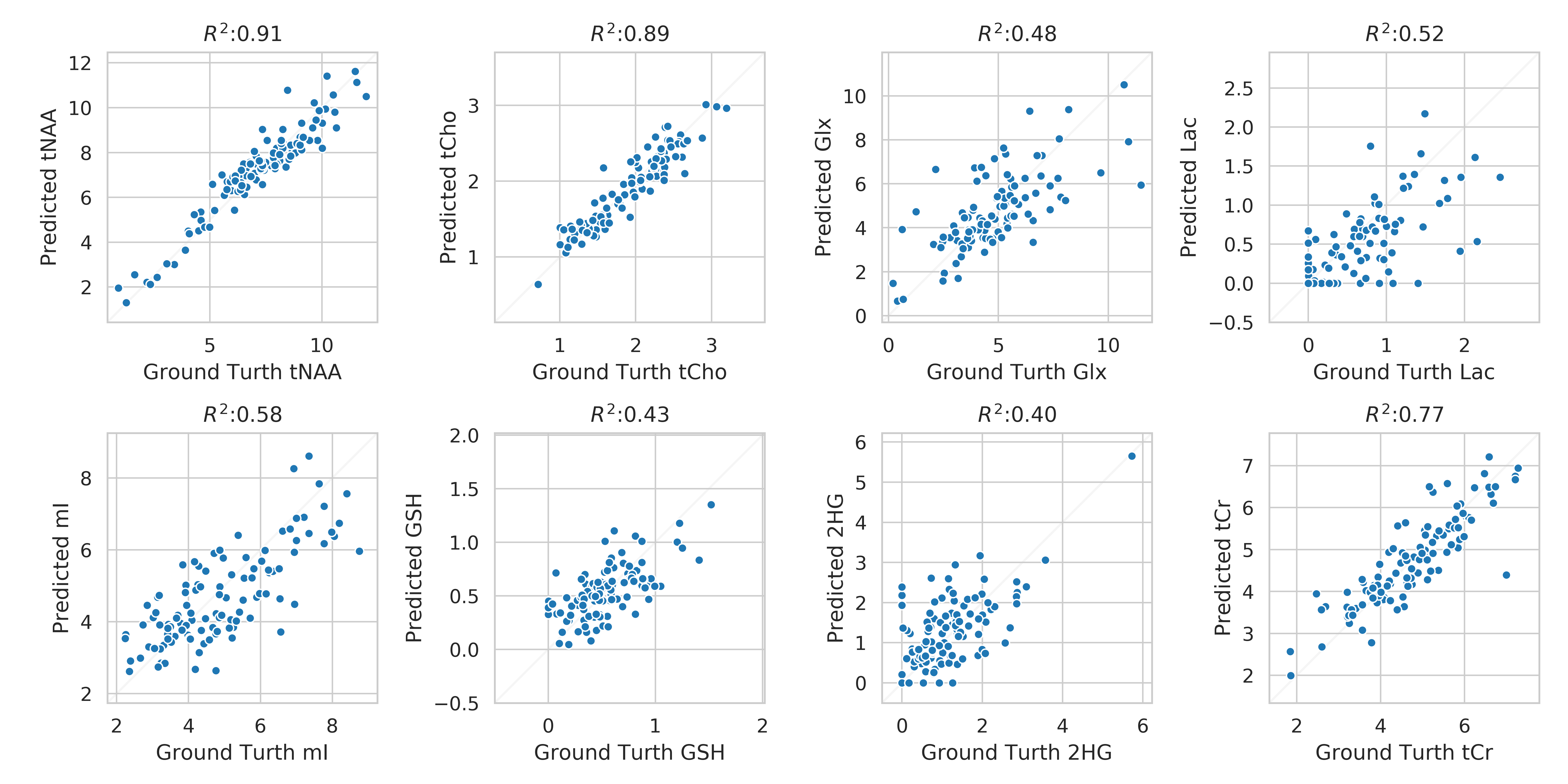
Correlation of metabolite concentration obtained using LCModel, for AE predicted and water suppressed spectra for the in-vivo test dataset. The x-axis shows the absolute concentration values estimated from water suppressed spectra and y-axis shows the corresponding AE predicted spectra. Overall, there is a strong correlation between metabolite for tNAA, tCho, tCr and Glx, Lac, GSH, mI and 2HG has a decent correlation. The clustering pattern seen in other metabolites can be caused by reconstruction error and change in the degree of freedom of LCModel fit between the spectra.