2414
Deblurring of spiral fMRI images using deep learning
Marina Manso Jimeno1,2, John Thomas Vaughan Jr.1,2, and Sairam Geethanath2
1Columbia University, New York, NY, United States, 2Columbia Magnetic Resonance Research Center (CMRRC), New York, NY, United States
1Columbia University, New York, NY, United States, 2Columbia Magnetic Resonance Research Center (CMRRC), New York, NY, United States
Synopsis
fMRI acquisitions benefit from spiral trajectories; however, their use is commonly restricted due to off-resonance blurring artifacts. This work presents a deep-learning-based model for spiral deblurring in inhomogeneous fields. Training of the model utilized blurred simulated images from interleaved EPI data with various degrees of off-resonance. We investigated the effect of using the field map during training and compared correction performance with the MFI technique. Quantitative validation results demonstrated that the proposed method outperforms MFI for all inhomogeneity scenarios with SSIM>0.97, pSNR>35 dB, and HFEN<0.17. Filter visualization suggests blur learning and mitigation as expected.
Introduction
T2*-weighted fMRI requires short acquisition times and efficient k-space sampling to accurately detect BOLD signal1 changes. Rapid sequences such as spirals or EPI acquire k-space using only a few long read-out shots. This feature makes them more susceptible to field inhomogeneities, resulting in artifacts that can be especially severe in brain regions where different tissue types interface2. Spiral trajectories are less motion-sensitive, provide shorter readout times, and improve signal recovery in some brain areas compared to EPI2. Despite their benefits, spiral use in fMRI is limited mainly due to off-resonance induced image blurring.Multiple off-resonance correction methods exist, e.g., any version of Conjugate Phase Reconstruction (CPR)3 or iterative reconstruction techniques4. However, they can suffer from inaccurate corrections at regions of severe field inhomogeneity and long, demanding, and complex computation5. Thus, these methods become impractical when correcting fMRI data that entails hundreds of whole-brain coverage time series. This study aims to demonstrate the feasibility of a deep-learning network for spiral deblurring at different inhomogeneity ranges for its application on spiral-based fMRI.
Methods
We utilized resting-state 3T EPI images and field maps from 10 subjects6 (OpenNeuro, ds000224) with a resolution of 64x64x34. We forward-modeled the EPI images using the field map and a 3-shot spiral trajectory of 9.6 ms readout duration to simulate blurring (Figure 1). Data augmentation was analogous to Lim et al.5 and included scaling the field map by 𝛼 and adding an offset 𝛽 to reproduce diverse inhomogeneity ranges.The network architecture (TensorFlow-Keras7) was a 2D U-net8 consisting of 23 ReLU activated convolutional layers (4 for downsampling) and 4 deconvolutional upsampling layers. The loss functions aimed to minimize structural (Structural Similarity Index loss) and voxel-wise differences (L1 loss, MSE loss) and to preserve edge information (gradient loss).
Pre-processing included normalizing between [0, 1] and resizing images to 128x128. The generated dataset consisted of five time-points selected randomly and corrupted with a different 𝛼-𝛽 combination. The training-validation-testing split was 90-5-5%. We trained two models for 150 epochs to investigate the field map’s effect, using only the blurred slice as input and using both the blurred slice and the field map. The total number of training slices was 1624.
Validation experiments compared the models’ deblurring performance with Multi-Frequency Interpolation (MFI)9 using peak-SNR, SSIM, and High-Frequency Error Norm (HFEN)10. We also visualized filter activations. As a testing experiment, we attempted to deblur spiral PRESTO-based brain images.
Results
Figure 2 shows how the blurring of a validation slice increases with 𝛼 and the absolute value of 𝛽 since they broaden the field map’s frequency range. The maximum and minimum field map values obtained were 838 and -980.25 Hz. All correction techniques successfully deblurred all images. Quantitative results (Figure 3) demonstrated that U-net correction outperforms MFI with SSIM greater than 0.97 and pSNR values larger than 35 dB for all images. Both U-net models display similar performance metrics, with the model trained without field map showing slightly higher pSNR in four out of five cases. HFEN minimum values correspond to the U-net corrections. From here on, the results shown come from the U-net trained without field map.Filter activations (Figure 4) of test slices revealed that the model picked up the blurring induced by the spiral sampling and off-resonance and removed it from the image while enhancing edge sharpness. Evaluation results (Figure 5) of the model on a PRESTO dataset demonstrated the model’s capability to emphasize the image’s edges, as the output-input difference image conveys. However, it also magnified other artifact-related high-frequency information such as phase artifacts due to RF spoiling errors.
Discussion
The parameters 𝛼 and 𝛽 mimic inhomogeneous fields and the effect of improper shimming5. It is essential to train the model in a broad frequency range as the actual acquisition inhomogeneity is unknown beforehand. Furthermore, spiral artifacts worsen as the off-resonance range increases.SSIM results demonstrate high structural fidelity; pSNR metrics indicate high-quality correction, and HFEN values convey that the model restores the image’s high spatial frequency features after deblurring. Compared to MFI, U-net results show better quantitative metrics, and it is faster. Moreover, we demonstrated that a field map is not required for DL deblurring to perform satisfactorily. This is a significant advantage since field map acquisition increases scan duration and may lead to errors if the image registration is not accurate.
Filter visualization suggests that the encoding half of the model identifies blurring, and the decoding half removes it while detecting edges and sharpening them. The evaluation results demonstrated that the model amplifies artifacts in the input image, conveying limited tolerance to other non-blurring artifacts. The PRESTO T2* contrast of the dataset is different from the training contrast, which may also affect correction performance.
Future work includes increasing the number of slices in the test/train dataset, comparing U-net results to calibrationless iterative reconstruction methods, evaluating in a spiral non-PRESTO dataset, and investigating the effect of blurring and deblurring in downstream functional connectivity analysis.
Conclusion
The proposed method for DL-based deblurring of spiral fMRI images in field ranges of up to ±1000 Hz outperformed MFI on simulated data visually and quantitatively. Filter visualization suggested successful deblurring and high-frequency feature enhancement.Acknowledgements
This study was funded [in part] by the Seed Grant Program for MR Studies and the Technical Development Grant Program for MR Studies of the Zuckerman Mind Brain Behavior Institute at Columbia University and Columbia MR Research Center site.References
- J. E. Chen and G. H. Glover, “Functional Magnetic Resonance Imaging Methods,” Neuropsychol. Rev., vol. 25, pp. 289–313, 2015.
- G. H. Glover, “Spiral imaging in fMRI,” Neuroimage, vol. 62, no. 2, pp. 706–712, 2012.
- D. C. Noll, C. H. Meyer, J. M. Pauly, D. G. Nishimura, and A. Macovski, “A Homogeneity Correction Method for Magnetic Resonance Imaging with Time-Varying Gradients,” IEEE Trans. Med. Imaging, 1991.
- B. P. Sutton, D. C. Noll, and J. A. Fessler, “Fast, iterative image reconstruction for MRI in the presence of field inhomogeneities,” IEEE Trans. Med. Imaging, 2003.
- Y. Lim, Y. Bliesener, S. Narayanan, and K. S. Nayak, “Deblurring for spiral real-time MRI using convolutional neural networks,” Magn. Reson. Med., vol. 84, pp. 3438–3452, 2020.
- E. M. Gordon et al., “Precision Functional Mapping of Individual Human Brains,” Neuron, vol. 95, no. 4, pp. 791–807, 2017.
- M. Abadi et al., “TensorFlow: A system for large-scale machine learning,” in Proceedings of the 12th USENIX Symposium on Operating Systems Design and Implementation, OSDI 2016.
- O. Ronneberger, P. Fischer, and T. Brox, “U-net: Convolutional networks for biomedical image segmentation,” in Lecture Notes in Computer Science (including subseries Lecture Notes in Artificial Intelligence and Lecture Notes in Bioinformatics), 2015.
- L. C. Man, J. M. Pauly, and A. Macovski, “Multifrequency interpolation for fast off-resonance correction,” Magn. Reson. Med., vol. 37, no. 5, pp. 785–792, 1997.
- S. Ravishankar and Y. Bresler, “MR image reconstruction from highly undersampled k-space data by dictionary learning,” IEEE Trans. Med. Imaging, vol. 30, no. 5, pp. 1028–1041, 2011.
Figures

Figure 1. Spiral blurring simulation. We used EPI resting-state fMRI data and corresponding field maps to simulate spiral blurring by sampling the images with a spiral trajectory of three shots and readout duration of 9.6 ms. Data augmentation included field map range alteration using combinations of 𝛼=(1, 1.25, 1.5, 1.75, 2) and β=(-100, -50, 0, 50, 100) Hz.
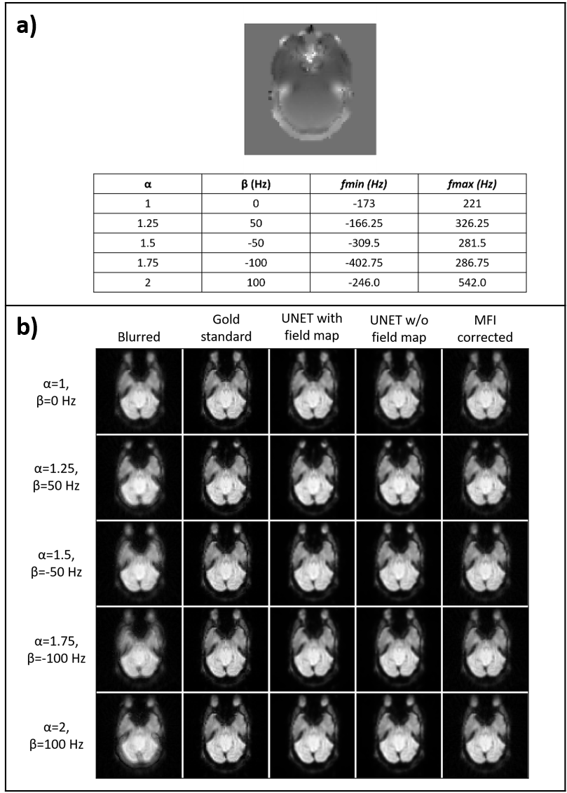
Figure 2. Validation results. Field map augmentation modified the frequency range of each slice depending on the parameters 𝛼 and β. a) shows the different combinations for an example slice and the achieved frequency ranges. b) Image panel displaying the blurred image, gold standard, U-net correction with field map, U-net correction without field map, and MFI correction images.
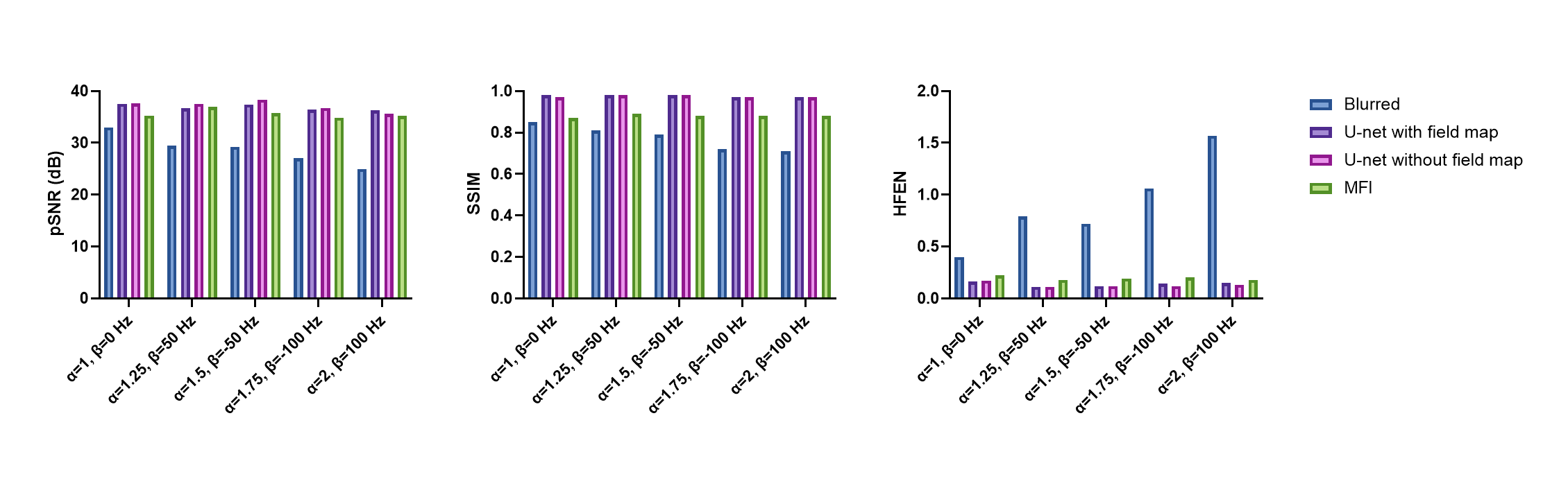
Figure 3. Quantitative validation results. pSNR, SSIM, and HFEN results corresponding to the blurred, U-net with field map corrected, U-net without field map corrected, and MFI corrected images in Figure 2 for five different off-resonance frequency ranges.

Figure 4. Filter visualization. Visualization of representative filters from the 2nd, 5th, 22nd, and 25th convolutional layers for four different brain slices from the testing dataset for model explainability.
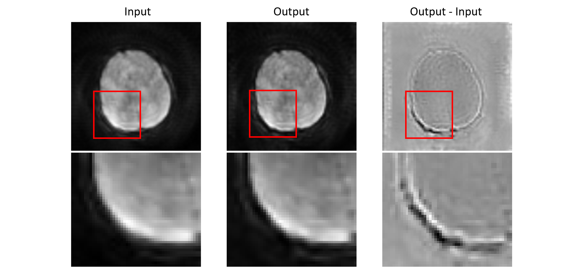
Figure 5. Evaluation experiment result. Slice and magnified region (red square) from a spiral fMRI PRESTO acquisition (left), deep-learning deblurring model correction of the image (middle), and output-input difference image (right).