INTRODUCTION

Parkinson’s disease (PD) is a chronic progressive movement disorder¹. An estimated 12.9 million people will suffer from PD worldwide by 2040. Deep grey matter structures are involved in the pathophysiology of PD. To date, many studies still use manual or semi-automated approaches to demarcate the substantia nigra (SN) and other nuclei. Automatic segmentation may facilitate the quantitative analysis of these structures and improve the reliability of the results. We proposed a deep learning method to simultaneously segment the caudate nucleus (CN), globus pallidus (GP), putamen (PUT), red nucleus (RN), and SN in both hemispheres from quantitative susceptibility mapping (QSM) data.

METHODS

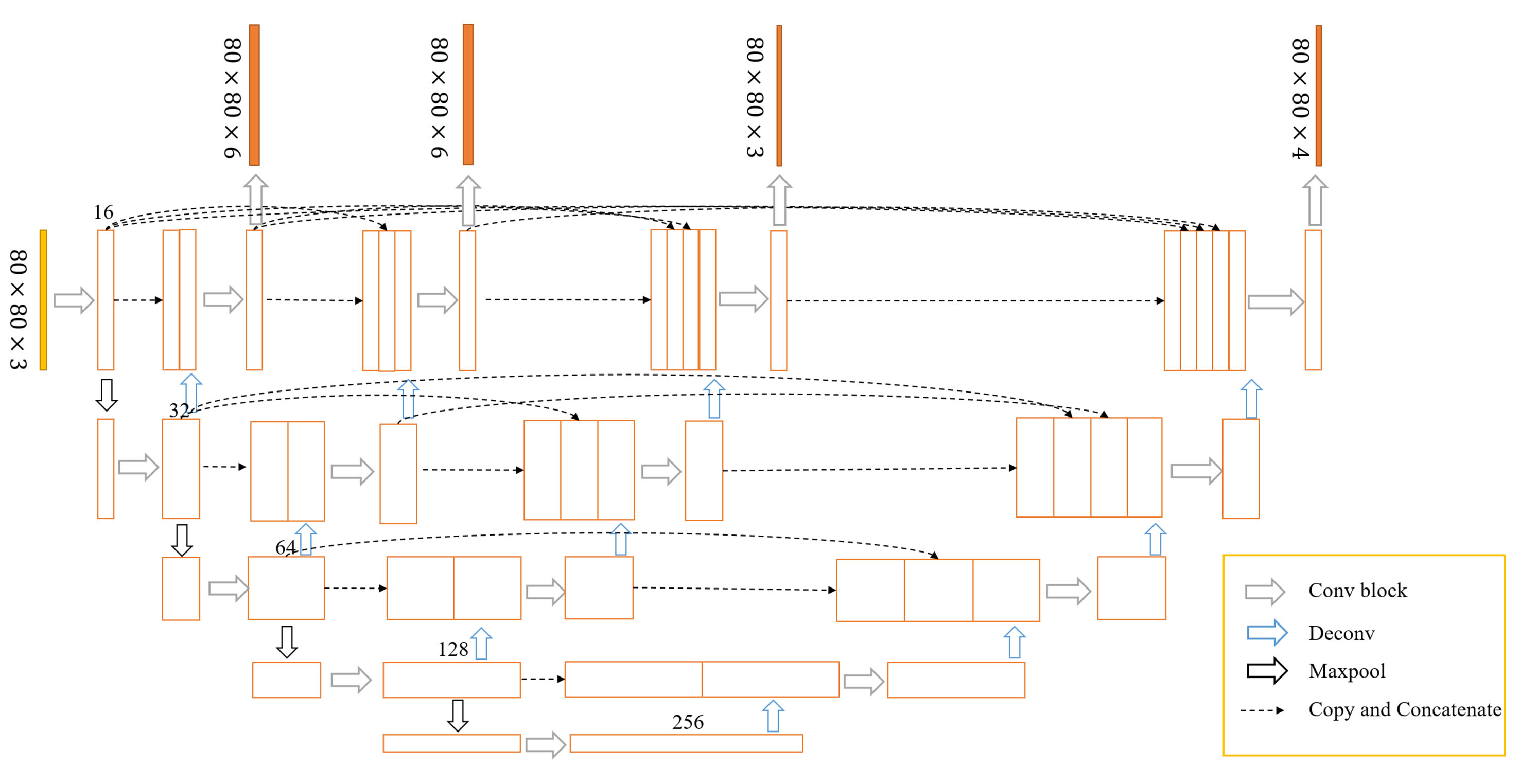
This study was approved by the local Institutional Review Board and all subjects signed a consent form. A total of 230 cases were collected on two 3T scanners (Ingenia, Philips Healthcare, Eindhoven, The Netherlands) with the same 15-channel head coil. A seven-echo 3D GRE sequence was used with: TE = 7.5 ms and ΔTE = 7.5 ms, TR = 62 ms, flip angle = 30˚, pixel bandwidth = 174 Hz/pixel, matrix size = 384 × 144, slice thickness = 2 mm, and in-plane resolution = 0.67 mm × 1.34 mm. All scans were acquired along the anterior commissure-posterior commissure (AC-PC) line. The QSM process included the following steps: a brain extraction tool (BET) was applied (threshold = 0.2, erode = 4 and island = 2000) using the first echo magnitude data; followed by a 3D phase unwrapping with 3DSRNCP, and sophisticated harmonic artifact reduction (SHARP) to remove unwanted background fields; and, finally, an iterative approach to reconstruct the susceptibility maps². The regions of interest (ROIs) for CN, GP, PUT, RN and SN were manually drawn by experienced radiologists and used as the ground truth for segmentation.
The dataset was randomly split into training (184 cases) and validation (46 cases) cohorts. The 2.5D patch sized 80×80×3 was cropped according to the center of the image slice which contained the whole brain gray matter nuclei. Random augmentation strategy including shifting, rotation and shearing was applied for each sample and all samples were standardized using Z-score during training. We used the U-net++ model³ with deep supervision shown in Fig.1 to segment the brain nuclei regions. U-net++ consisted of an encoder to capture high-level semantic information and decoder path to recover spatial information with nested and dense skip connections. The model contained four output branches at different semantic levels and all predicted probability maps had the same resolution as the input. The large variations of shape and scale of brain nuclei was a challenge for predicting the five nuclei regions simultaneously. In order to address this problem, in the first two output branches, the model generated six regions including five nuclei and the background; in the third branch, the model generated three regions including the SN, RN, and background; in the last branch, the model generated four regions including the CN, GP, PUT, and background.
The combination of Dice and Tversky loss⁴ was used as the loss function to address the pixel imbalance of foreground and background:
$$Dice(P，G)=\frac{2|P\cap G|}{|P|+|G|}$$
$$Tversky(P，G,\alpha,\beta)=\frac{|PG|}{|PG|+\alpha|P\backslash G|+\beta|G\backslash P|}$$
$$loss= 1-Tversky(P，G,\alpha,\beta) + 1-Dice(P, G)$$
where P and G represents prediction and ground truth, respectively. Hyper-parameters α and β were set to 0.7 and 0.3 in the experiments.
During the training process, an early stopping strategy was applied to handle overfitting and the training was aborted if the loss on the validation dataset did not reduce over 20 epochs. The Adam algorithm was applied to minimize the loss function during the back-propagation process with an initial learning rate of 10⁻³. The models were implemented using TensorFlow (version: 2.0.0) and Python (version: 3.7). The experiments were conducted on a workstation equipped with four NVIDIA TITAN XP GPUs. For validation, standardized patches were fed into the trained model to segment five brain nuclei regions. The predicted probability maps of the third and last output branches were binarized (threshold set as 0.5) to obtain the final results, before they were evaluated with Dice coefficients (DSC).

RESULTS

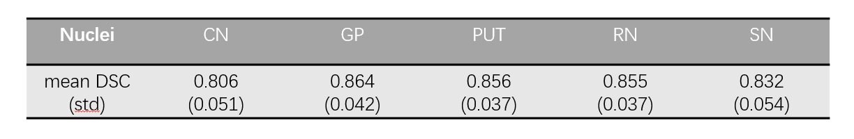
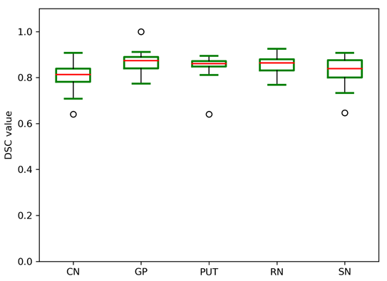
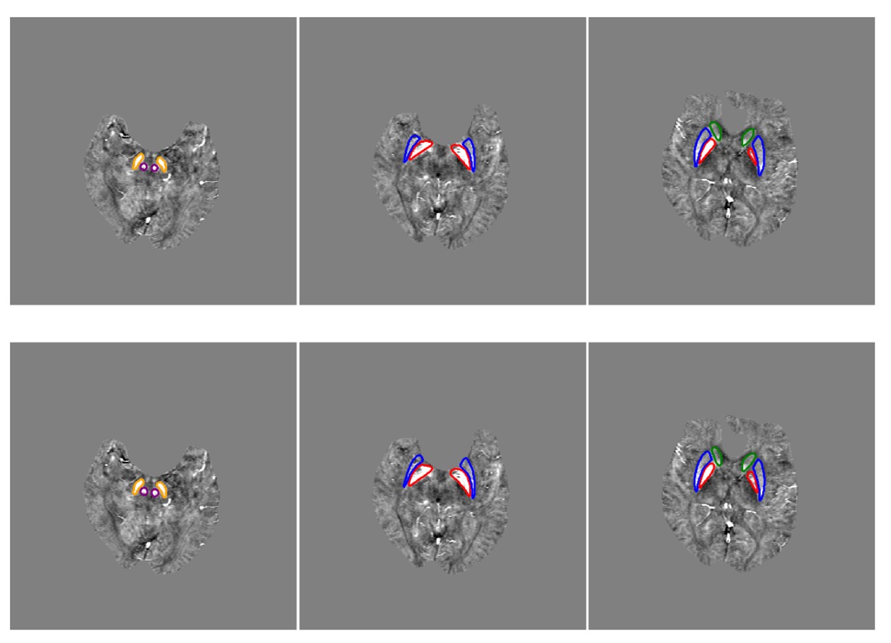
In the validation dataset, the segmentation model achieved a mean DSC of 0.806 ± 0.051, 0.864 ± 0.042, 0.856 ± 0.037, 0.855 ± 0.037, and 0.832 ± 0.054 (Table 1) for CN, GP, PUT, RN, and SN regions, respectively. Fig. 2 showed the distribution of the DSC values for the automatic segmentation. From the comparison between segmented regions and ground truth (Fig. 3), the U-net++ is seen to accurately segment the five nuclei.

DISCUSSION AND CONCLUSION

Segmentation of all the five nuclei achieved a mean DSC value above 0.8, thus the trained model could accurately segment brain nuclei regions on QSM images. The 2.5D patches provided inter-slice information which improved segmentation performance. The nested and dense skip connections in the U-net++ model reduced the semantic gap between encoder and decoder stage. The use of deep supervision from different semantic level features led to better segmentation accuracy. In conclusion, the proposed model achieved high quality segmentation of the CN, GP, PUT, RN and SN on QSM images. With the QSM technique increasingly applied to clinical diagnosis and scientific research, future studies are expected to benefit from such automated and robust segmentation methods.

Acknowledgements

None