2401
A Supervised Artificial Neural Network Approach with Standardized Targets for IVIM Maps Computation
Alfonso Mastropietro1, Daniele Procissi2, Elisa Scalco1, Giovanna Rizzo1, and Nicola Bertolino2
1Istituto di Tecnologie Biomediche, Consiglio Nazionale delle Ricerche, Segrate, Italy, 2Radiology, Northwestern University, Chicago, IL, United States
1Istituto di Tecnologie Biomediche, Consiglio Nazionale delle Ricerche, Segrate, Italy, 2Radiology, Northwestern University, Chicago, IL, United States
Synopsis
Fitting the IVIM bi-exponential model is challenging especially at low SNRs and time consuming. In this work we propose a supervised artificial neural network approach to obtain reliable parameters estimation as demonstrated in both simulated data and real acquisition. The proposed approach is promising and can outperform, in specific conditions, other state-of-the-art fitting methods.
Introduction
IVIM is a bi-exponential model to explore diffusion and perfusion tissue properties starting from a set of multi b-values MRI diffusion weighted images [1]. IVIM has several possible applications in clinical and preclinical research, but the fitting process is challenging especially when working with low SNR images and time consuming. Bayesian methods offer a better quality than least square fitting algorithm at the expense of longer computational time [2], but the employment of artificial intelligence algorithms can push forward the reliability of the data and boost the application of IVIM in the medical field. The purpose of this work is to employ an artificial neural network trained on numerical phantoms for IVIM maps computation, to test its performance and to compare it with a state-of-the-art Bayesian method and the other artificial intelligence algorithms proposed in the literature [3,4]. We also employed the trained network for the computation of IVIM maps on an in-vivo mouse brain.Methods
SimulationsNumerical phantoms were generated using a MatLab R2020a custom made script. Starting from physiologically typical mammal brain D values in the range [0.0005-0.002 mm2/s], D*[0.005-0.1] and f [0.025-0.4], diffusion weighted images were computed for different b-values (0, 25, 50, 75, 100, 150, 300, 800, 1000 s/mm2) using the formula below:
$$S(b)=S_{0}\times(1-f)\times e^{-b\times D}+f\times e^{-b\times D^{*}}$$
Rician noise was added to create the final diffusion weighted images with different SNRs (10, 25, 50, 100, 150, 200). 2000 numerical phantoms were generated for each SNR value. The Shepp-Logan phantom was used in our simulations; each region of interest was characterized by a randomly generated parameters triplet.
In-vivo Animal Data
Experimental procedures involving animals complied with Northwestern’s IACUC guidelines. MRI acquisitions were performed on 7T ClinScan MRI scanner (Bruker, Germany) equipped with a 12 cm diameter gradient coil system (max strength 115 mT/m) using a four-channel phase-array receiver coil. A volume quadrature coil was used for transmission. The imaging protocol included a multiple b-values (bs =0, 25, 50, 75, 100, 150, 300, 800, 1000) SE-EPI diffusion weighted images (TR/TE=3500/27 ms, flip-angle=90, averages=4, slice-thickness=1 mm, voxel-size=0.282x0.282 mm2).
Neural Network
Using MatLab Machine Learning toolbox, we implemented a three hidden layer feed-forward neural network with 9 nodes for each layer and a linear activation function. The training was performed using Levenberg-Marquardt backpropagation algorithm and mean square root error as loss function. The network was trained using the first 1000s simulated images for each SNR, splitting the data 70/15/15 % for training/validation/test data. Training data and the real value were standardized before neural network training. We trained the network using data for each SNR data set separately. A total number of 6 networks were trained.
Analysis
The trained network was used to compute D, f and D* of the remaining 1000 simulated images for each SNR. We computed a map for parameter for each SNRs data set using the network trained with same SNR value. IVIM maps were also generated using a state-of-the-art Bayesian method [2], an unsupervised neural network approach as proposed by Barbieri et al [3] and a supervised method as proposed by Bertleff et al [4]. The methods were implemented as described in each specific paper. We tested the results from the different computation methods in multiple ways: visually inspecting few randomly sampled simulated data, computing the average/median percentage error voxel-wise, investigating how the error change based on parameters range, and applying the proposed method to an in-vivo mouse dataset to assess if the quality of the obtained results is in line with what we found in simulations.
Results
SimulationsFig 1 shows examples of D, f and D* maps generated with our neural network model and their respective ground-truth images.
Fig 2 shows errors distribution for all parameters at each different SNRs. As clearly shown, most of the errors are close to 0 for each parameter. However, some outliers are shown especially for f and D*.
In Figure 3 a quantitative comparison between our ANN approach and the other implemented methods is shown. Considering both the average and median errors, the proposed method performs in most condition better than the Bayesian approach and the other ANNs methods.
In vivo animal data
Our approach showed the best performance in-vivo using networks trained with images having SNR similar to that of the input images. In our case, a mean SNR of 70 characterized the in-vivo images and taking into consideration brain symmetry and the comparison with Bayesian generated maps the best fitting was obtained using the ANN trained with images having SNR 100. An example is shown in Figure 4.
Conclusion
In this work we demonstrated that the proposed neural network architecture is a valuable alternative tool for the computation of IVIM parameters. Based on our analysis we suggest that the ANN method described in this abstract offers improved results when compared to state-of-the-art Bayesian approaches, especially when using data/images with low SNR. In addition once the network is trained the computation process to extract quantitative maps requires few seconds (depending on matrix size and hardware performance). The method is promising for in vivo applications even when compared to other similar approaches based on ANNs [3,4].Acknowledgements
No acknowledgement found.References
- Le Bihan, D. (2019). What can we see with IVIM MRI?. Neuroimage, 187, 56-67.
- Gustafsson, O., Montelius, M., Starck, G., & Ljungberg, M. (2018). Impact of prior distributions and central tendency measures on Bayesian intravoxel incoherent motion model fitting. Magnetic Resonance in Medicine, 79(3), 1674-1683.
- Barbieri, S., Gurney‐Champion, O. J., Klaassen, R., & Thoeny, H. C. (2020). Deep learning how to fit an intravoxel incoherent motion model to diffusion‐weighted MRI. Magnetic resonance in medicine, 83(1), 312-321.
- Bertleff, M., Domsch, S., Weingärtner, S., Zapp, J., O'Brien, K., Barth, M., & Schad, L. R. (2017). Diffusion parameter mapping with the combined intravoxel incoherent motion and kurtosis model using artificial neural networks at 3 T. NMR in Biomedicine, 30(12), e3833.
Figures
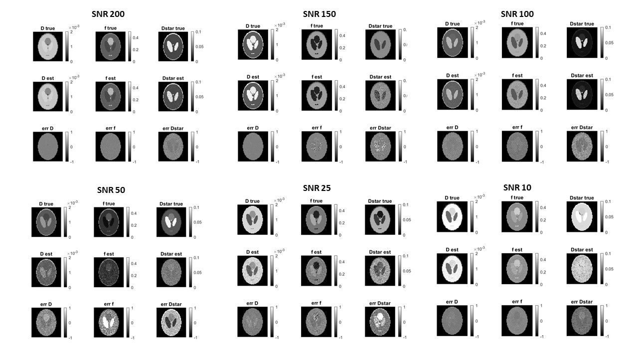
Fig.1: The image shows a representative examples of D, f and D* maps for each SNRs, in simulations, generated with our neural network model and their
respective ground-truth images.
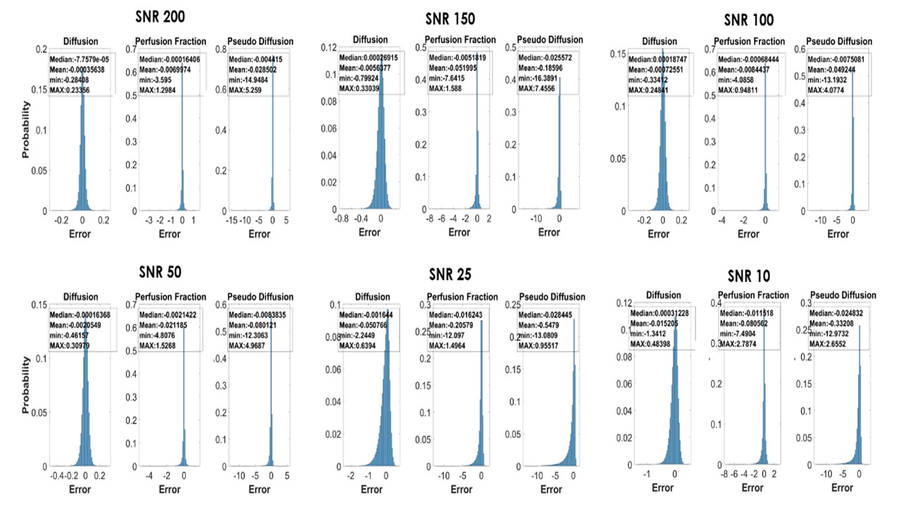
Fig.2: The image shows errors distribution for all parameters at each
different SNRs. As clearly shown, most of the errors are close to 0 for each
parameter. However, some outliers are shown especially for f and D*.
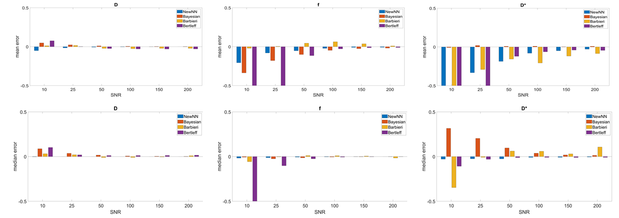
Fig.3: The image shows a quantitative comparison between our ANN
approach and the other implemented methods. Considering both the
average and median errors, the proposed method performs in most conditions
better than the Bayesian approach and the other ANNs methods. y axis range was set from -0.5 to 0.5.
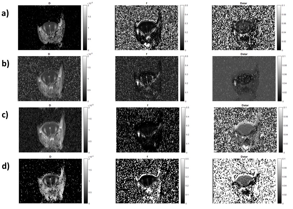
Fig.4: The image shows in-vivo IVIM maps examples generated using: our neural network a), Bayesian method b), Barbieri's neural network c), and Bertleff's neural network d).