Introduction

Intravoxel Incoherent Motion (IVIM) MR imaging is a diffusion weighted imaging technique that is sensitive to the diffusion of water in the parenchyma as well as flow-mediated diffusivity of microvascular blood (perfusion). Commonly, the fraction of microvascular perfusion in the IVIM signal $$$f_{perf}$$$ is calculated using a bi-exponential model. Recently, however, it was shown that besides the parenchymal diffusion and microvascular perfusion an additional, intermediate, component can be observed [1]. The fraction of the intermediate diffusion is suggested to be related to interstitial fluid in the perivascular spaces (PVS). PVS are associated with a number of disorder, ranging from Alzheimer’s disease, stroke and multiple sclerosis [2]. Therefore, estimating $$$f_{int}$$$ from IVIM data can provide valuable clinical insights. However, estimating $$$f_{int}$$$ can be challenging, since three-component models and spectral decompositions of the IVIM signal are dependent on the acquired b-values and signal-to-noise ratio (SNR). Therefore, in this study we will examine several b-value sampling strategies for measuring the $$$f_{int}$$$ using simulated IVIM data.

Methods

Numerical simulations

Ground-truth IVIM data with three components were computationally synthesized using the IVIM signal decay equation:

$$\frac{S(b)}{S(0)}=\frac{f_{par}E_{1,par}E_{2,par}e^{-bD_{par}}+f_{int}E_{1,int}E_{2,int}e^{-bD_{int}}+f_{perf}E_{1,perf}E_{2,perf}e^{-bD_{perf}}}{f_{par}E_{1,par}E_{2,par}+f_{int}E_{1,int}E_{2,int}+f_{perf}E_{1,perf}E_{2,perf}}$$

Where, $$$E_{1,k}=(1-2e^{-\frac{TI}{T_{1,k}}}+e^{-\frac{TR}{T_{1,k}}})$$$, with $$$k=par$$$ or $$$int$$$; $$$E_{1,perf}=(1-e^{-\frac{TR}{T_{1,perf}}})$$$; $$$E_{2,k}=e^{-\frac{TE}{T_{2,k}}}$$$, with $$$k=par$$$, $$$int$$$ or $$$perf$$$; and $$$f_{par}=1-f_{int}-f_{perf}$$$.

The IVIM parameters used to simulate the signal decay were $$$f_{int}= .050$$$; $$$f_{perf}=.022$$$; $$$D_{par}=7.15\cdot10^{-4}$$$mm²/s; $$$D_{int}=2.4\cdot10^{-3}$$$mm²/s and $$$D_{perf}=1.63\cdot10^{-2}$$$mm²/s; corresponding to normal appearing white matter (NAWM). Additionally, data with high $$$f_{int}$$$ were synthesized simulating white matter hyperintensities (WMHs) using $$$f_{int}= .271$$$; $$$f_{perf}= .024$$$; $$$D_{par}=8.93\cdot10^{-4}$$$mm²/s; $$$D_{int}=2.0\cdot10^{-3}$$$mm²/s and $$$D_{perf}=7.85\cdot10^{-2}$$$mm²/s [1][3]. The following relaxation times were used; $$$T_{1,par}=1081$$$ms, $$$T_{2,par}=95$$$ms, $$$T_{1,pef}=1624$$$ms, $$$T_{2,perf}=275$$$ms, $$$T_{1,int}=1250$$$ms, $$$T_{2,int}=1500$$$ms [1][4-7].

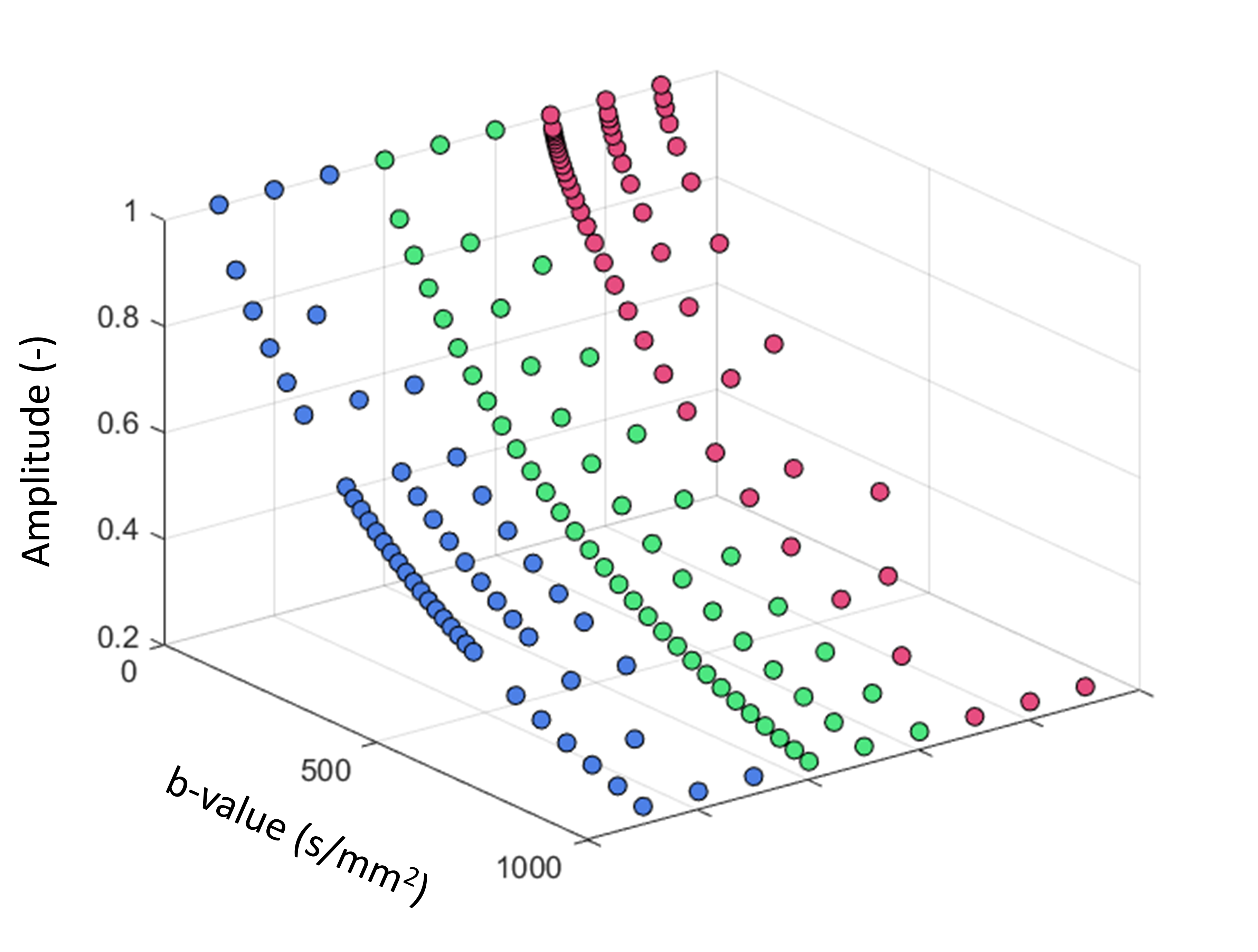
To estimate the effects of acquired b-values on the quantification of $$$f_{int}$$$, 1000 Gaussian noise realizations were calculated for nine sets of b-values and an SNR of 100 (defined as the signal at b = 0s/mm² divided by the standard deviation of the noise). Each of the b-values sets that are considered range from 0 to 1000s/mm². Three sets were linearly spaced, three were logarithmically spaced, and three had an oversampling in the range of 300<b<600s/mm² where $$$b\cdot D_{int}\approx1$$$. The number of b-values is varied for each sampling strategy (10, 15 and 30). Figure 1 graphically depicts the nine schemes with different b-values.

Fitting method

The NNLS uses a predefined basis set A with M exponential decays to characterize the measured signal $$$y$$$ as; $$$y_i=\sum_j^Ms_je^{-b_iD_j}=\sum_j^M \mathbf{A}_{ij}s_j,i=1,2,..,N$$$ where $$$s_j$$$ is the amplitude corresponding to the $$$D_j$$$ diffusivity, $$$b_i$$$ is the measured signal of b-value $$$i$$$ and $$$N$$$ represents the total number of b-values. Now, the NNLS problem can be written as, $$$\chi_{min}^2=\min_{s \geq 0}(\sum_{i=1}^N\mid\sum_{j=1}^M\mathbf{A}_{ij}s_j-y_i\mid^2)$$$ where $$$\chi_{min}^2$$$ represents the misfit that is minimized by the NNLS algorithm. Typically, the number of b-values is smaller than the elements in the basis set (N<M) making the NNLS an ill-posed problem. To provide a more stable solution, a regularized version of the NNLS can be used, adding a smoothing constraint, $$$\chi_{reg}^2=\min_{s \geq 0}(\sum_{i=1}^N\mid\sum_{j=1}^M\mathbf{A}_{ij}s_j-y_i\mid^2+\mu\sum_{j=1}^M\mid s_{j+2}-2s_{j+1}+s_j\mid^2)$$$ where $$$\mu$$$ is the regularization parameter and $$$\chi_{reg}^2$$$ is the regularized misfit [8].

A basis set with 120 logarithmically spaced elements ranging from 0.1$$$\cdot$$$10^-3 to 1000$$$\cdot$$$10^-3 is used. Subsequently, the $$$f_{int}$$$ is defined as the amplitude fraction of the $$$D_j$$$ elements in the range of 1.5$$$\cdot$$$10^-3 to 4.0$$$\cdot$$$10^-3. The $$$f_{int}$$$ is corrected for the effects of inversion and relaxation [1].

Validation

The accuracy of the different strategies was evaluated using the bias, $$$\hat{f_{int}}-f_{int}$$$, where $$$\hat{f_{int}}$$$ is the mean estimated intermediate fraction, and $$$f_{int}$$$ is the ground-truth intermediate fraction.
The precision of the different strategies was evaluated by the standard deviation of the estimated intermediate fraction.

Results

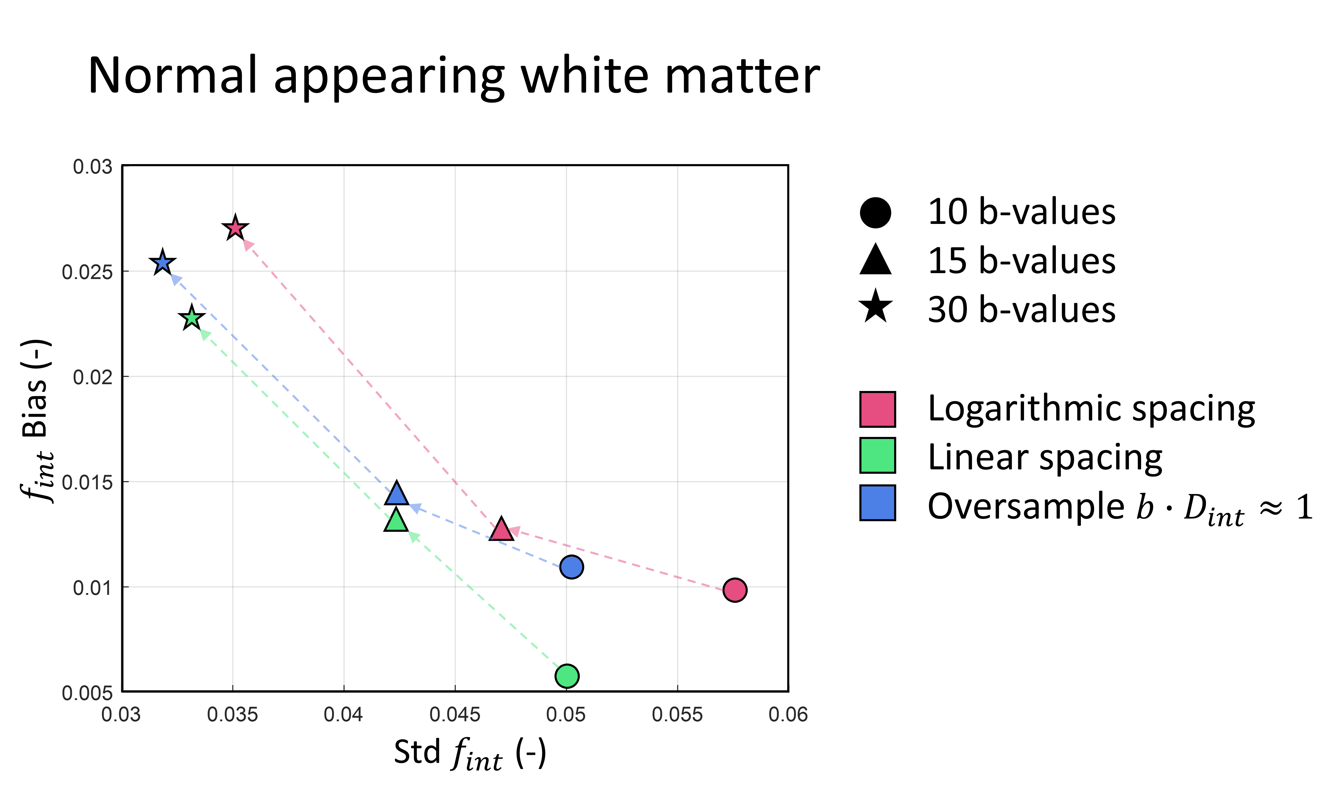
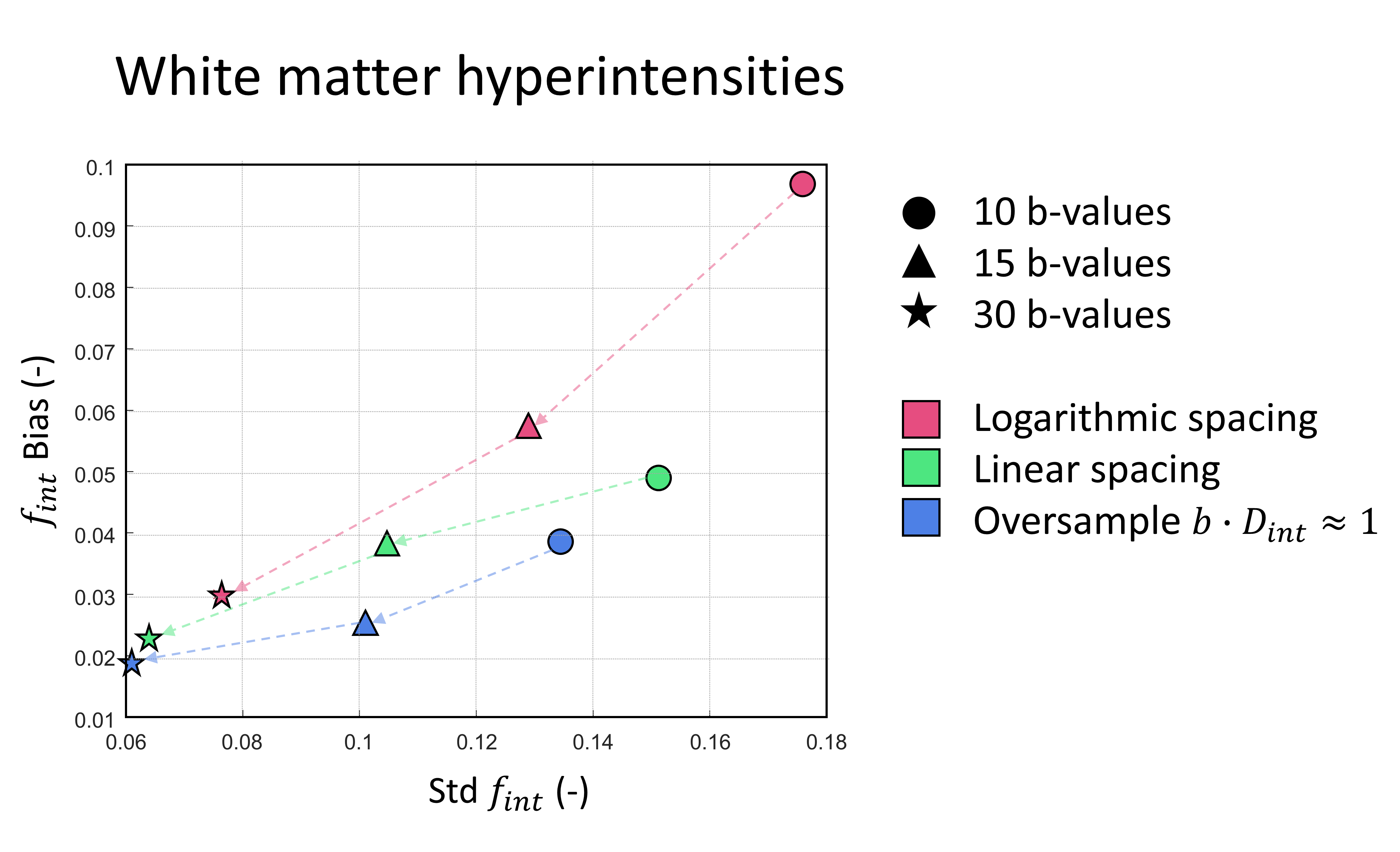
The accuracy and precision of the $$$f_{int}$$$ estimation in terms of bias and standard deviation is shown in figure 2 for the NAWM and in figure 3 for the WMHs. For the NAWM a linear spacing of the b-values seems to provide the best trade-off between accuracy and precision. However, for the WMHs, where a large $$$f_{int}$$$ is present, oversampling the $$$b\cdot D_{int}\approx1$$$ range provides the highest accuracy and precision.

Discussion & Conclusion

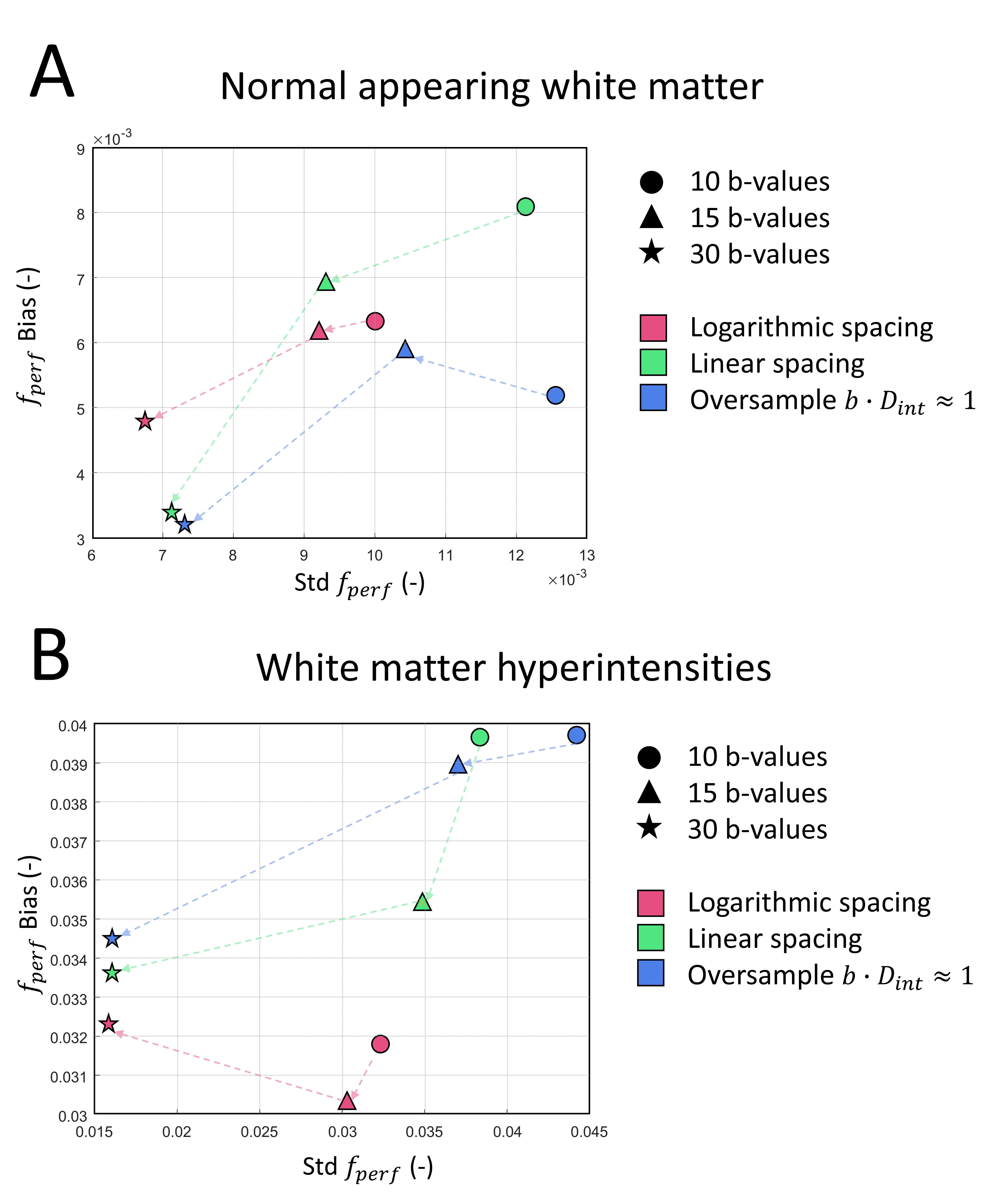
Interestingly, acquiring more b-values does not appear to be valuable in the NAWM, as the accuracy drops, while in the WMHs acquiring more b-values does relate to better performance. This can be explained; when simulating data with 10 b-values, for roughly 14% of the noise realizations no third component is found, artificially lowering the measured $$$f_{int}$$$. The third component is absent in 6% of the realizations with 15 b-values, and in less than 1% in the 30 b-values case. This effect, combined with a systematic over-estimation of the $$$f_{int}$$$, results in the presented behavior. Over-estimation of the intermediate fraction can be contributed to an under-estimation of the $$$D_{par}$$$ and $$$f_{par}$$$, which is a known phenomenon related to the logarithmic distribution of the basis set [9].

When a large intermediate diffusion component is present in the IVIM signal (e.g. in WMHs), b-value sampling strategies specifically aimed to quantify this component can provide a better estimate of $$$f_{int}$$$ compared to linearly or logarithmically spaced b-values. However, studies interested in measuring $$$f_{perf}$$$ benefit more from logarithmically spaced b-values (which oversamples $$$b\cdot D_{perf}\approx1$$$ range), while a linearly spaced b-value set provides a good trade-off between $$$f_{int}$$$ and $$$f_{perf}$$$ (Figure 4A&B).

Acknowledgements

No acknowledgement found.