Introduction

An accurate assessment of myelin content poses a challenge to in vivo neurological MRI. There are a few approaches allowing one quantitatively or qualitatively to evaluate the amount of myelin water in the brain, but most of them are based on indirect myelin measures^1,2. It is still a challenge to quantify myelin directly and the developed methods are limited for in vivo clinical applications³ due to their time consuming implementation. One of the most frequently used approaches is based on a multi-echo T₂ (MET2) measurement modelling for at least two water pools with different T₂ relaxation times, namely, myelin water trapped between the myelin bilayers and intra- and extra-axonal water². A major problem in MET2 is that the fitting algorithms used for the estimation of the model parameters are highly vulnerable to noise and imaging artefacts⁴. In the present work, we suggest an optimised MET2 framework providing an increase in precision and accuracy of MWI assessments. This is accomplished by using noise⁵ and Gibbs-ringing⁶ correction steps and Bayesian estimator⁷ allowing one significantly to accelerate the computations.

Methods

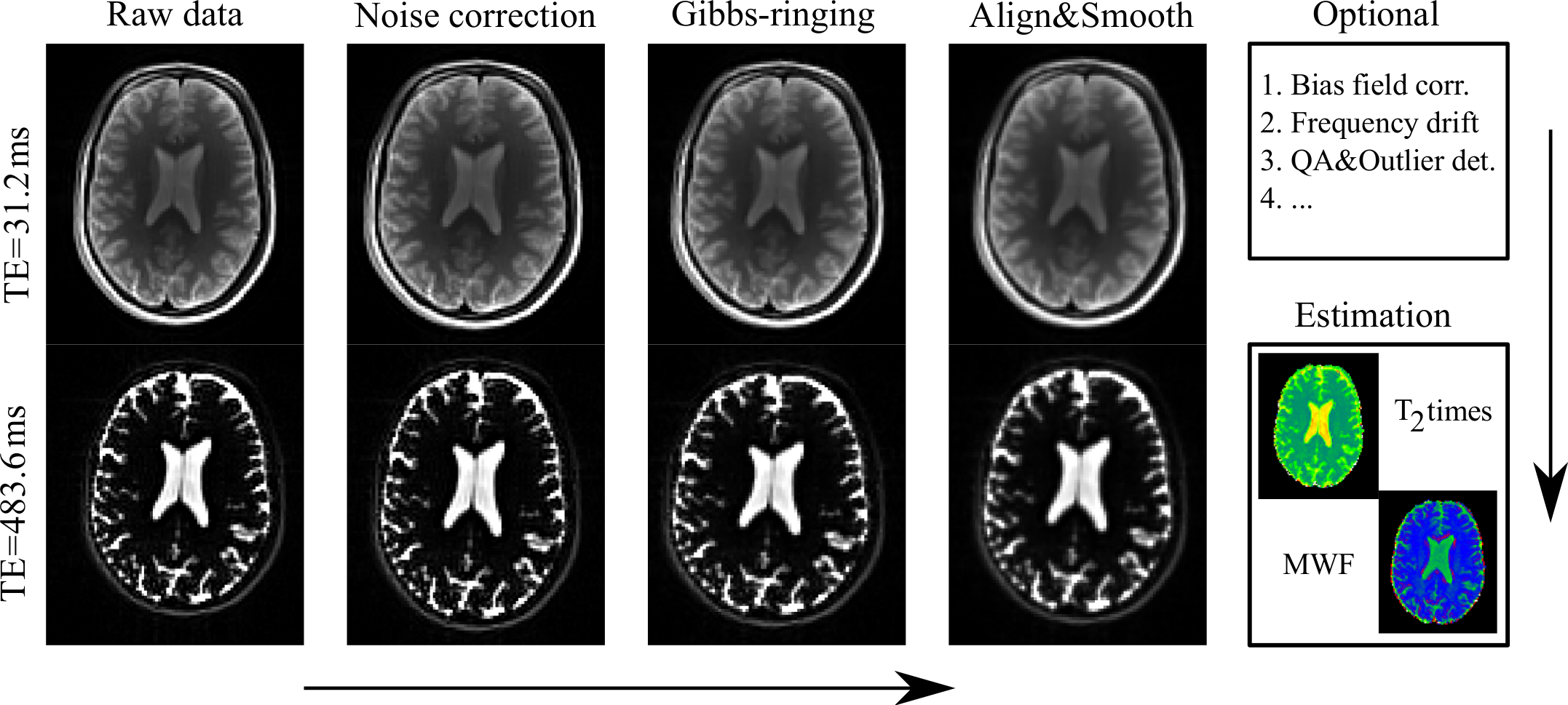
A scheme of the optimised framework is presented in Fig. 1 and consists of two major parts. First data preparation and pre-processing including at least three basic steps: noise correction based on removal of noise-only principle components⁵, Gibbs-ringing correction for all images⁶, and all volume normalisation, including a Gaussian smoothing with small kernel. Second the estimation of the myelin water fraction by means of a Bayesian estimation. Other steps such as a bias field correction, frequency drift, gradient non-linearities correction etc. can be included as well.
This is based on the idea of modelling the signal decomposition by the assumed parameter distribution⁷. The MET2 signal decay is simulated for many parameters using the following representation:
S = v₁exp(-t/T_M) + v₂exp(-t/T_A) + v₃exp(-t/T_CSF),
where ∑v_i=1are the fractions of myelin water (M), intra- and extra-axonal water (A), and cerebrospinal fluid (CSF), respectively. The simulated signal is distorted by a non-central χ² noise. The Bayesian estimation is defined as a maximisation of a posteriori probability p as
x(f) = argmax p(x|f),
where x is the parameter set of relaxation model, and f is the signal features. The simulations establish the training set allowing us to find an optimised set of polynomial regressors solving the optimisation problem. For a comparison, we used a standard fitting approach based on non-negative least squares^2,4,5.
After signed informed consent prior to the participation, we measured 32 years old healthy male volunteer. Imaging was performed on a 3T Prisma scanner (Siemens Healthcare, Erlangen, Germany). In vivo MET2 data consist of 32 echos with the TE step equals to 15.6 ms. Image resolution is 2 mm³. Repetition time is 5.06 s.

Results

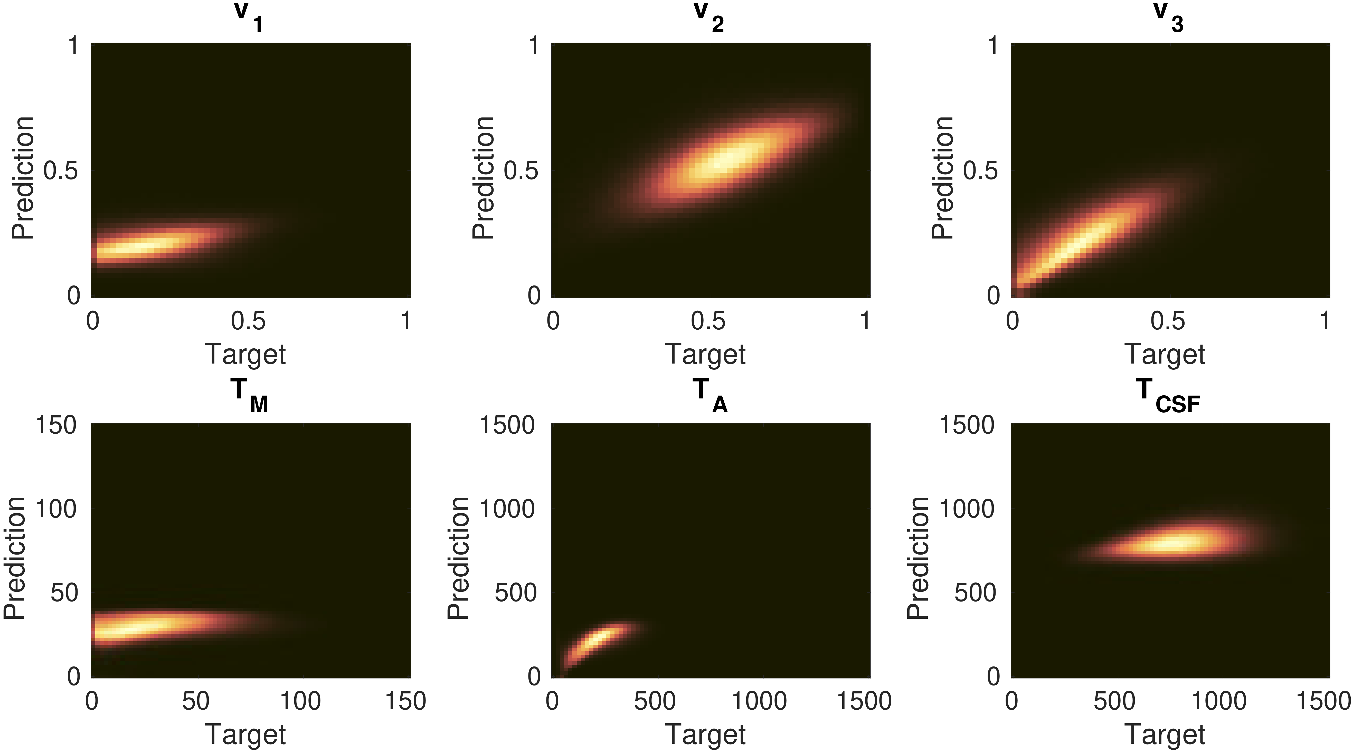
In Fig. 2 we present the correlation results of model training using simulations with the Gaussian distributions G (mean, std) of all parameters:
v₁ = G (10, 30); v₂ = G (70, 30); v₃ = G (20, 30); T_M = G (15, 30)ms; T_A = G (200, 100)ms; T_CSF = G (800, 200)ms.
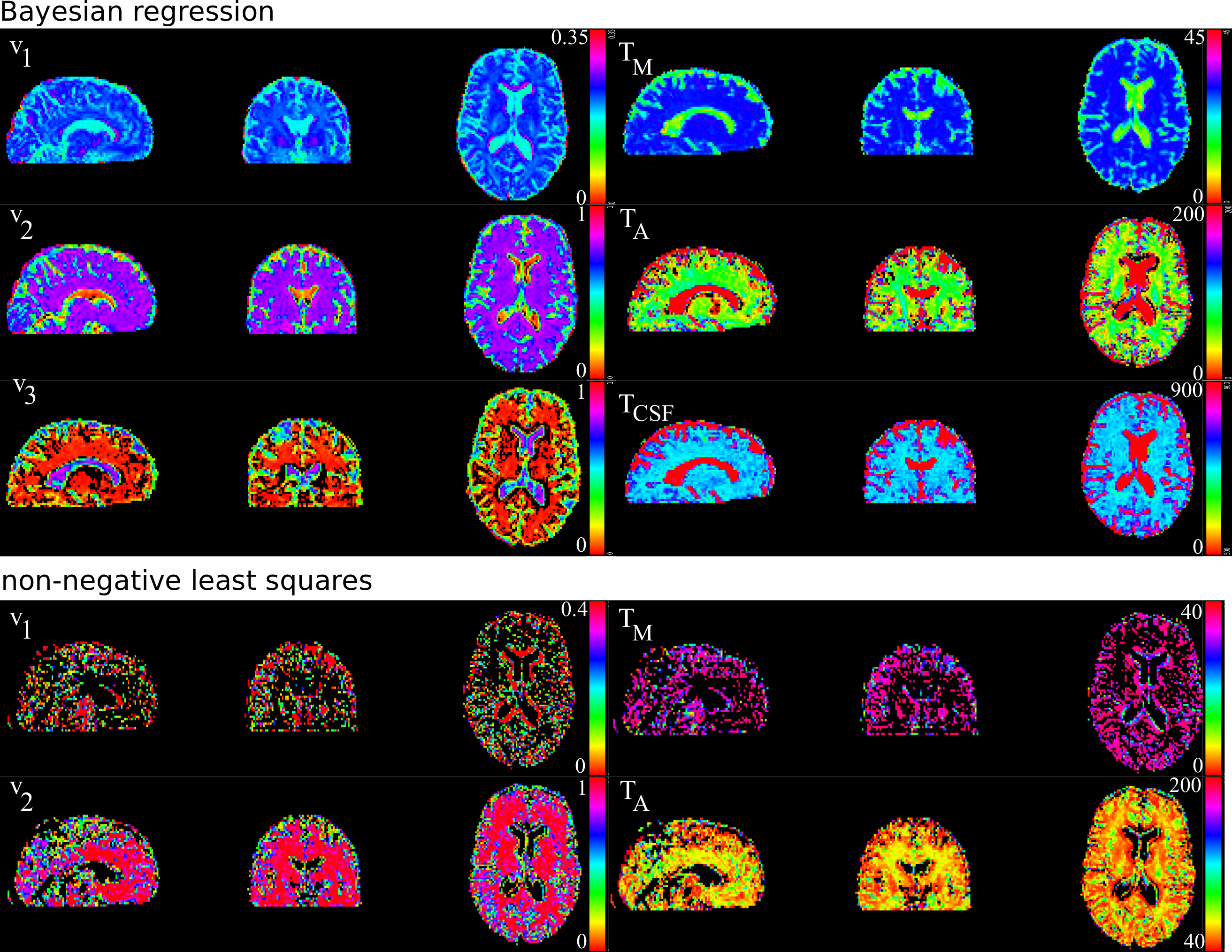
Typical values used for the water fractions and relaxation times in the simulations were found in the literature^1,2. Notably, a creation of training sets and computing of the Bayesian estimator is performed on a laptop within minutes. As a result, the following estimation of the myelin water fraction and the related relaxation times for in vivo data takes a few seconds. Fig. 3 presents the images of myelin related maps estimated by the Bayesian regression and non-negative least squares⁴.

Discussion and conclusion

The presented framework with a Bayesian regression approach is very fast and simple method for myelin water imaging. The developed optimised framework keeps a quite wide range of options for the myelin model representation by choosing different signal behaviour, noise level, and parameter distributions. The computational superiority and simplicity of the implementation allows one to use the Bayesian regression and proposed pipeline as a helpful tool in myelin model development and clinical research.

Acknowledgements

This work was funded by the Research Council of Norway (249795).