2288
Experimental validation of simulated implant heating induced by switched gradient fields1Physikalisch-Technische Bundesanstalt (PTB), Berlin, Germany, 2IRCCS Istituto Ortopedico Rizzoli, Bologna, Italy, 3Istituto Nazionale di Ricerca Metrologica (INRIM), Torino, Italy
Synopsis
Switching MR gradients induce eddy-currents in metallic implants. Gradient-aggressive MR sequences were used on a commercial 3 T scanner to heat orthopaedic prostheses ex vivo. Heating experiments are presented, and the measured temperature evolution is compared with corresponding numerical results. Numerical simulations have been successfully validated for five MR sequences at different implant position and orientations in the gradient field.
Introduction
The goal of this work is to evaluate the reliability of hazard assessments, performed via numerical simulations, for patients carrying orthopaedic metallic implants exposed to MR gradient fields. While heating produced by radiofrequency (RF) has been investigated intensively [1-3], only few studies address heating of implants by switched gradients [4-6]. This work aims to complement simulation results based on [7,8] by experiments designed to maximize absolute accuracy. Clinically relevant MR conditions were chosen for gradient coil (GC), gradient sequence, implant type, and position.Experimental Methods
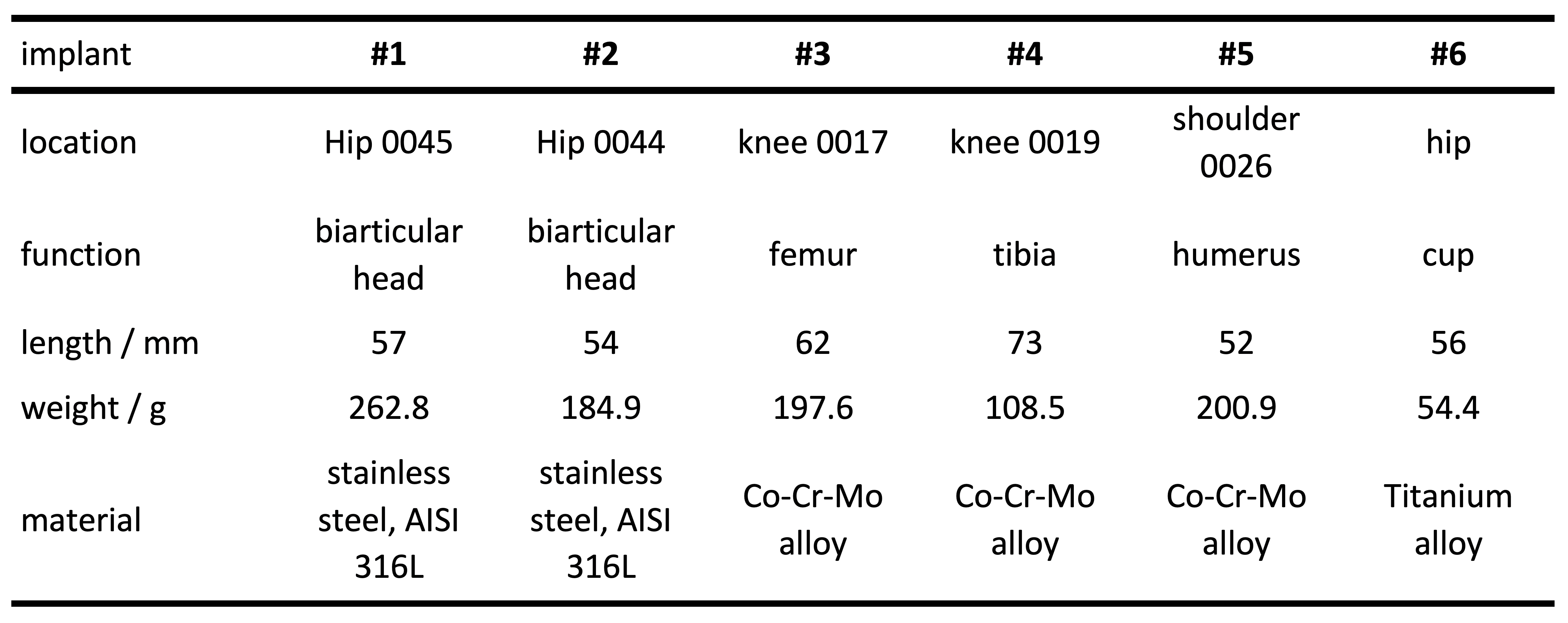
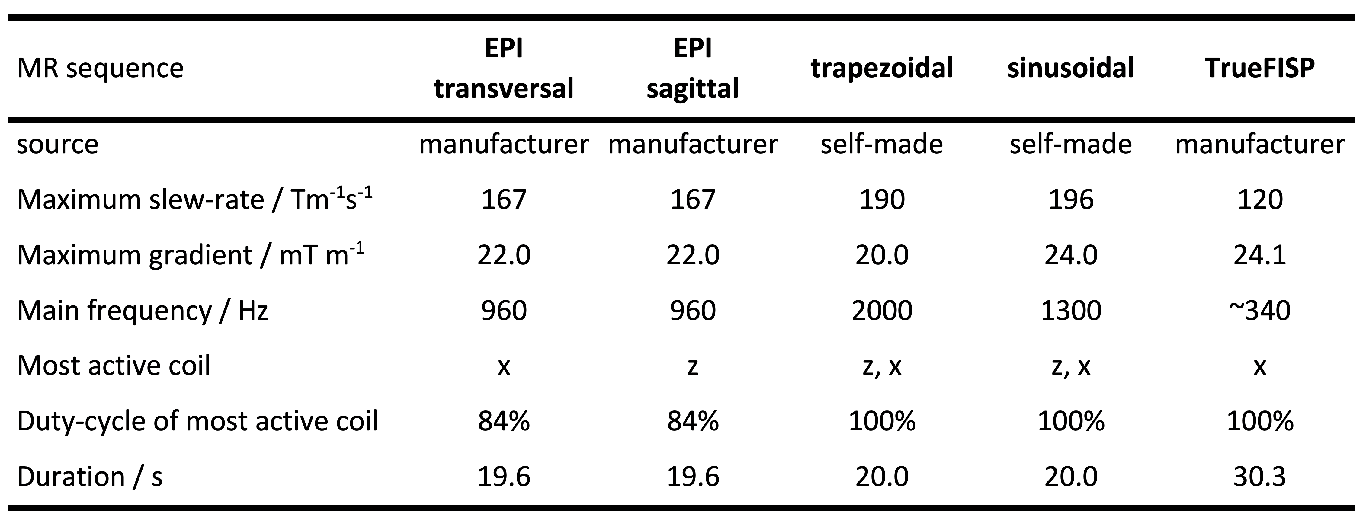
Six orthopaedic prostheses (Table 1) were analysed. They were placed at various realistic orientations and positions inside a 3 T scanner (Siemens Verio) and encapsulated in a polystyrene box. The scanner was operated in normal mode and with minimal RF power. The evolution of implant temperature was recorded for various MR sequences (Table 2). Gradient-coil currents were recorded and denoised to be used in simulations. Three NTC thermistors (diameter 0.5 mm, length 3 mm) with twisted leads were used as temperature sensors. An active low pass filter with cut-off frequency at 10 Hz filtered the signal of a Wheatstone-Bridge. At the end of the day, the sensors were calibrated with a calibrated PT100 thermometer. Whenever possible, blind holes were drilled into the implants to optimize sensor contact. Alternatively, an aluminium socket carrying the sensor was glued to the implant.Numerical Methods
The measured physical dimensions of the prostheses were used to build voxel models at 1 mm resolution. Simulations were performed at implant position $$$z=300 \text{ mm}$$$ and $$$250 \text{ mm}$$$ since the manufacturer supplied gradient-coil-field map shows a B-field maximum at $$$z=300 \text{ mm}$$$. Spatial power density distribution within the implant due to the GC field was computed following the approach described in [7]. The consequent heating was simulated by adopting a finite difference method with a Douglas–Gunn time split implemented to increase the computational efficiency [8]. Simulations allowed to determine the time evolution of temperature increases in the positions where sensors were located in the experiments.Results and Discussion
Compared to fibre-optical thermometers, NTCs offer huge advantages in terms of precision and speed but are susceptible to electromagnetic fields. Direct eddy-current heating of sensors was determined to be below 2 mK and the noise at MR condition $$$0.5 \text{ mK} / \sqrt{\text{Hz}}$$$ . Implants were repeatedly heated with different MR sequences for 20 s or 32 s followed by cooling periods of 200 s. A linear baseline was subtracted from the experimental data. Uncertainties of the baseline cause negligible errors < 2 mK during heating but lead to diverting temperatures at the end of the cooling period of up to 30 mK and to 12 mK in Fig 1.The implants used here were selected with a preference for large cross sections to induced eddy currents. A hip implant’s biarticular head was chosen for the first simulation because it promises the smallest uncertainty in eddy current simulation due to its simple geometry and well-known material properties in contrast to fine structured or porous implants.
Fig 1a shows the temperature evolution at 3 sensor positions in implant #1 (Table 1) during a sagittal EPI sequence for 20 s (Table 2). To quantify the deviation between experiment and simulation we use the root mean square of the temperature difference of all 3 sensors at $$$t=20 \text{ s}$$$. In the case of Fig 1 that is 0.021 K (4.6 % of temperature rise). The same metric applied to other 13 experiments with different positions in the GC, sequences, and orientations results in 0.057 K (8 %). Compared to the estimated experimental uncertainty of 15 % the deviation is rather small. Deviations in the cooling period increase with time. We attribute them to an imperfect baseline subtraction and roughly estimated heat loss coefficient of 3.5 W/(m2 K) . Since model validation does not depend on data at $$$t>40 \text{ s}$$$ , this is not a problem.
Fig 1b shows the temperature distribution at $$$t=20 \text{ s}$$$ and the asymmetry causing the difference of the sensors on the rim.
Heating data for a femoral knee implant at various z positions are shown in Fig 2a. The implant was placed on the symmetry axis and heated by a trapezoidal z-gradient. The heating rate shows a quadratic dependency around $$$z = 0$$$, reflecting the $$$(z\frac{\text{d}G_z}{\text{d}t})^2$$$ curve. The maxima at $$$z = ±350 \text{ mm}$$$ are in good agreement with manufacturer-provided gradient maps.
Limitations
With a wall thickness of 3.5 mm the chosen hip implant is rather solid, and the model resolution of 1 mm seems sufficient. Most implants have finer structures, however, and the appropriate model resolution needs to be determined separately for every case. The analysis of experimental uncertainties is still incomplete regarding material properties and gradient-field non-linearities.Conclusion
Numerical results on gradient heating of an orthopedic implant were successfully validated for different implant positions and five MR sequences. Cooling mechanisms were not investigated but are identical to the extensively studied case of RF heating. Fully simulation-based safety assessments are a valid tool, therefore, to estimate the hazard of gradient-aggressive MR sequences to implant carriers.Acknowledgements
This work has received funding from the EMPIR programme, co-financed by the Participating States and from the European Union’s Horizon 2020 research and innovation programme, under grant number 17IND01 – MIMAS.References
- Liu Y, Chen J, Shellock FG, Kainz W. Computational and experimental studies of an orthopedic implant: MRI-related heating at 1.5-T/64-MHz and 3-T/128-MHz. J Magn Reson Imaging 2013;37:491-497.
- Powell J, Papadaki A, Hand J, Hart A, McRobbie D. Numerical simulation of SAR induced around Co-Cr-Mo hip prostheses in situ exposed to RF fields associated with 1.5 and 3 T MRI body coils. Magn Reson Med 2012;68:960-968.
- Winter L, Seifert F, Zilberti L, Murbach M, Ittermann B. MRI-related heating of implants and devices: A Review. J Magn Reson Imaging 2020; Early View, https://doi.org/10.1002/jmri.27194.
- Graf H, Steidle G, Schick F. Heating of metallic implants and instruments induced by gradient switching in a 1.5-Tesla whole-body unit, J Magn Reson Imaging, 2007;26,:1328–1333.
- Brühl R, Ihlenfeld A, Ittermann B. Gradient heating of bulk metallic implants can be a safety concern in MRI. Magn Reson Med 2017;77:1739–1740.
- Arduino A, Zanovello U, Hand J, Zilberti L, Brühl R, Chiampi M, Bottauscio O. Heating of hip joint implants in MRI: the combined effect of radiofrequency and switched-gradient fields. Magn Reson Med 2020; doi: 10.1002/mrm.28666
- Arduino A, Bottauscio O, Brühl R, Chiampi M, Zilberti L. In silico evaluation of the thermal stress induced by MRI switched gradient fields in patients with metallic hip implant. Phys Med Biol 2019;64:245006. doi: 10.1088/1361-6560/ab5428.
- Arduino A, Bottauscio O, Chiampi M, Zilberti L. Douglas–Gunn method applied to dosimetric assessment in magnetic resonance imaging. IEEE Trans Magn 2017;53:1-4. doi: 10.1109/TMAG.2017.2658021.
Figures
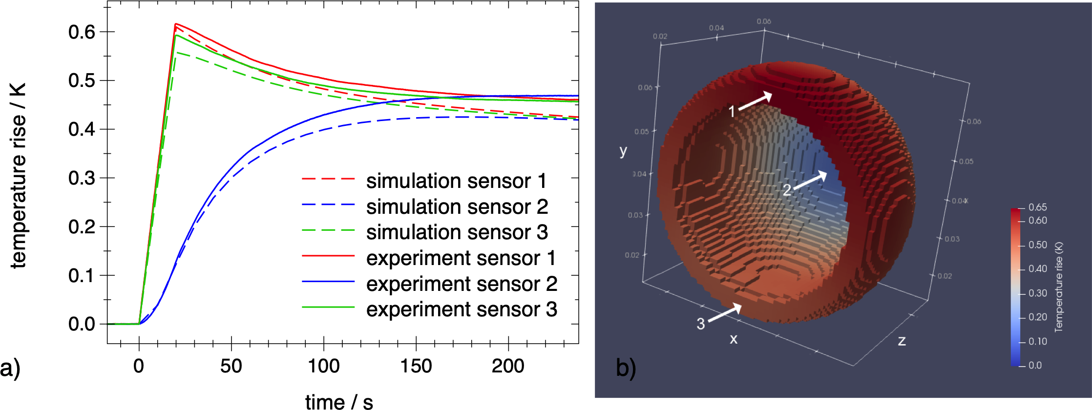
Fig 1a: Comparison of experimental (solid) and simulated (dashed) eddy-current heating of hip implant #1 at scanner coordinates $$$z=-300 \text{ mm}, y=-50 \text{ mm}, x=-145 \text{ mm}$$$. Central sensor in blue, sensors located on the rim in red and green. The EPI sequence was applied from $$$t=0 \text{ to } 20 \text{ s}$$$. The main eddy current circulates along the rim with its large cross section to the vector field $$$dB/dt$$$ of the read gradient z.
Fig 1b: Simulated temperature rise distribution at $$$t=20 \text{ s}$$$. The arrows indicate the sensor positions.
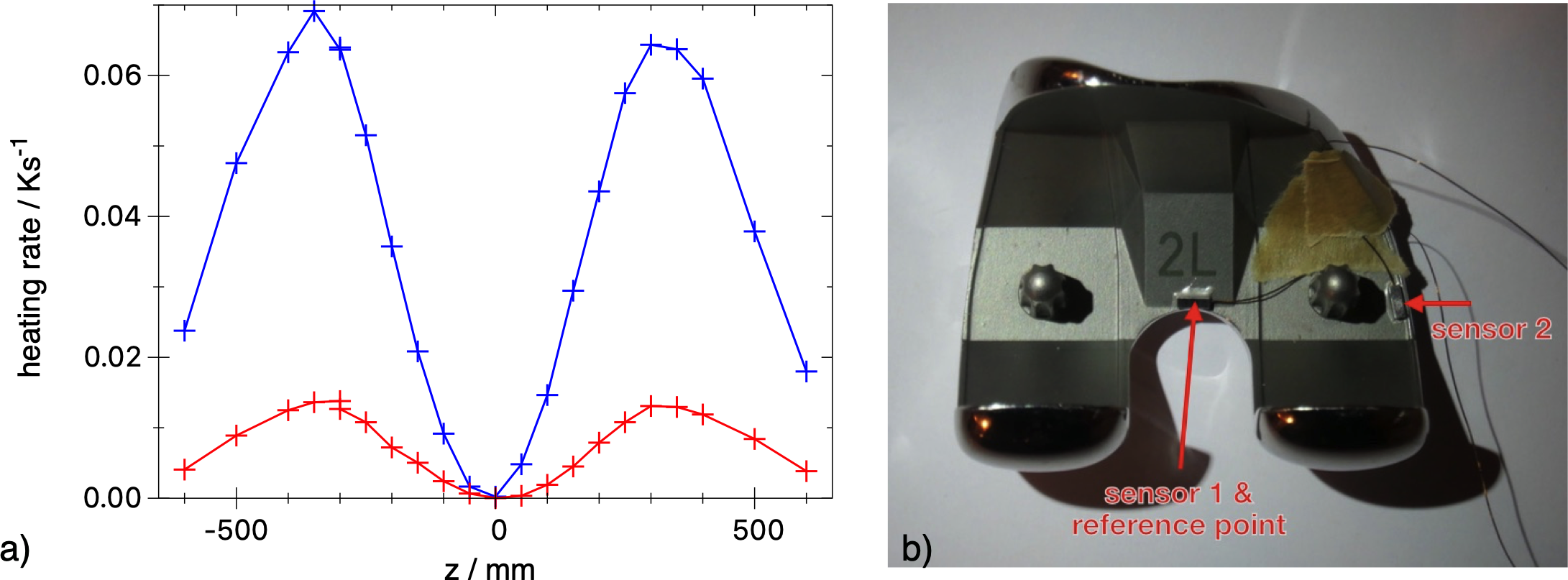
Fig 2a: Experimental heating rate of a knee implant #3 at $$$t=0, x=0, y=0$$$ and various $$$z$$$ positions in a clinically relevant orientation. The signal of the central sensor 1 is shown in blue, the lateral in red.
Fig 2b: An axial view of the knee implant with two NTC sensors mounted in sockets that are glued on the implant.