Introduction

Magnetic resonance spectroscopy (MRS) and spectroscopic imaging (MRSI) are techniques used to non-invasively provide information on the chemical composition of tissue in-vivo. MRSI is a technique that profiles the concentrations of metabolites in heterogeneous areas in the brain by acquiring a grid of spectra¹. However, analyzing larger areas of the brain through CSI is difficult because a large volume of data needs to be acquired at locations that contain different tissue components, namely white matter (WM), grey matter (GM), and cerebrospinal fluid (CSF). Due to these complexities, the investigator must look at many spectra which is very time-consuming. This work offers a way to compress and give an overview of the metabolic information obtained from an MRSI scan, specifically in WM and GM. Segmentation is a tool used to prevent inaccuracies in metabolite quantification in MRS by separating T1-weighted images into segmented GM, WM, and CSF images. WM and GM contribute most to the metabolite concentration in a voxel, while CSF has a negligible contribution. The software VDI is used to calculate the fractions of the three tissue types in each CSI voxel². Finally, the metabolic information is graphically represented through plots to describe how the relative concentrations differ with respect to the partial fractions.

Methods

Data collection: 46 MRSI scans of healthy control subjects were acquired at 3T (Siemens Skyra, Erlangen, Germany) using a semi-LASER sequence, TE/TR=40/1500, a 2D 16x16 matrix, and a voxel size of 10x10x15 mm3 (1.5 mL). These matrices correspond to a total of 2,944 voxels. T1-weighted anatomical volumes were also acquired using MPRAGE.
Data processing and quantification: MRSI scans were reconstructed using OpenMRS Lab and quantified using LCModel. FMRIB’s Automated Segmentation Tool (FAST) within the FSL library was then used to segment subject brain images into three tissue type classes, grey matter, white matter, and cerebrospinal fluid³. Visual Display Interface (VDI) software was used to calculate the fraction of WM, GM, and CSF in each MRSI voxel. Quantified metabolite ratios to total creatine (tCr) were obtained while selecting only voxels with a CRLB<50 and the innermost 7x7 voxel grid. Of the 46 controls, 16 were eliminated due to poor quality partial fraction maps which were due to low-resolution anatomical images and misalignment of the voxel grid. The metabolite ratios included: N-acetyl-aspartate (NAA), total choline (tCho), glutamate+glutamine (Glx), and myoinositol (mI). The white matter contribution by brain tissue to the metabolite ratios was defined as the concentration at which the WM partial fraction was 1.0 (WM_100%) or GM partial fraction was 0.0 (GM_0%), and for GM contribution, where WM partial fraction was 0.0 (WM_0%) or GM partial fraction was 1.0 (GM_100%). Partial fractions at each voxel were divided by the sum of WM and GM to remove the contribution of CSF.
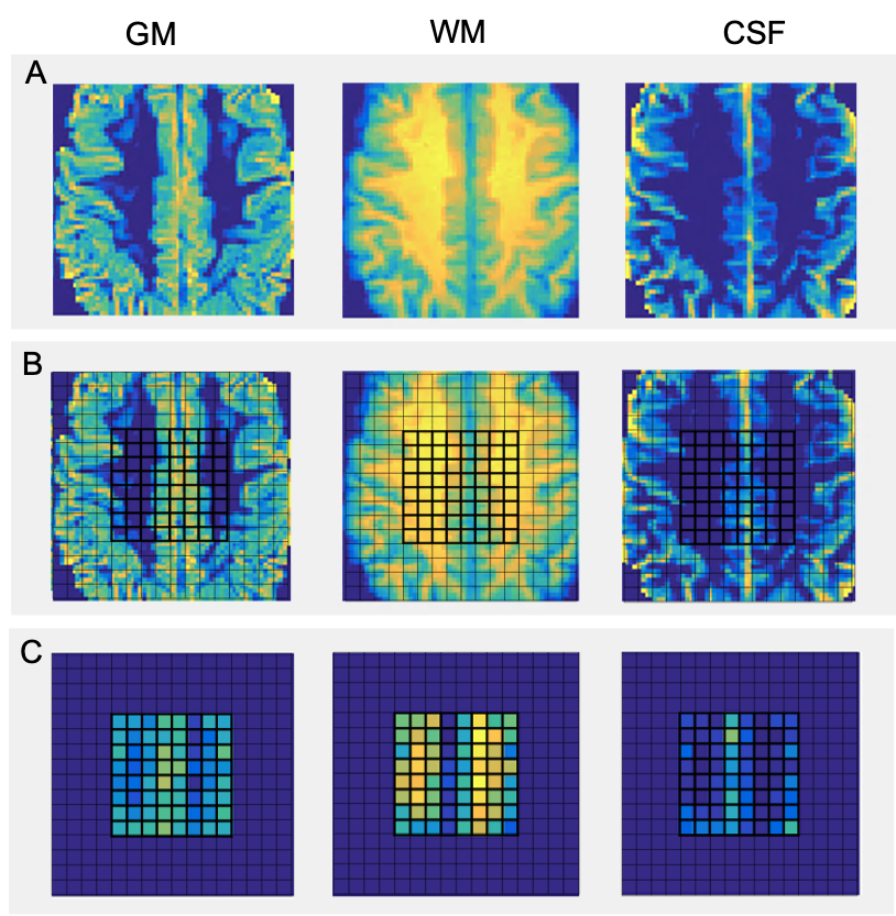
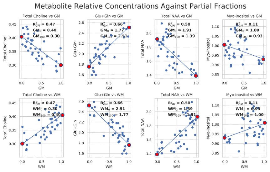
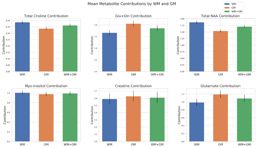
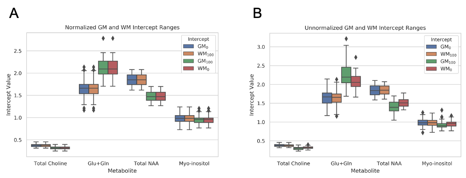
Data Visualization: All MRS scans were visualized by a 16x16 matrix of WM, GM, and CSF fractions which reconstructed an anatomical view of the brain. The partial fractions of WM and GM were plotted against metabolite ratios to creatine along with a linear fit to show correlation and extrapolate pure GM and WM metabolite contributions. The ranges of both normalized and unnormalized GM and WM contributions were visualized using boxplots. Finally, a histogram was used to compare mean contributions between GM and WM across different metabolites.

Results and Discussion

High-resolution images of the partial fraction maps of each tissue type give a clear view of anatomical features (Fig. 1). Scatterplots show the correlation of white and grey matter partial fractions in all MRSI voxels versus metabolite relative concentrations (Fig. 2). The contribution by purely WM (WM_100% and GM_0%) and by GM (WM_0% and GM_100%) are constant between WM and GM plots. Differences between GM and WM are shown in the bar plots for tNAA, tCho, and Glx, but not mI (Fig. 3). The boxplots show that within the two possible measurements for pure WM contribution (WM_100% and GM_0%), measurements from white matter (WM_100%) have a narrower range compared to grey matter (Fig. 4). When the dataset is normalized for only WM and GM, the contributions share similar medians and ranges. These ranges then provide a basis for comparing different cohorts for studies comparing metabolite differences in disease. Furthermore, the ranges provided in this set of healthy controls can serve as a normative reference with which individual data points could be plotted for precision clinical diagnosis. The advantage of this method is that voxel location does not have as large an effect. This method may also be sensitive to global metabolic changes due to disease. Results comparing a clinical cohort will be presented at the conference.

Conclusion

This work combines voxel segmentation performed on anatomical images with MR spectroscopic imaging to analyze the metabolic composition of pure GM and WM tissue via linear regression of individual metabolites. The methodology has the potential to improve the analysis of MRSI to study conditions that affect the chemical composition of the brain.

Acknowledgements

No acknowledgement found.