Introduction

The inhibitory neurotransmitter γ-aminobutyric acid (GABA) is a major target of ¹H-MRS studies in the human brain¹. Challenges are that GABA concentration is low (~1mM), and GABA signals are overlapped by other metabolites. GABA has been routinely quantified in ultra-high field, and short TE spectra^2-3, but there is a need to investigate the influence of LCModel fitting parameters on GABA quantification and sensitivity for detecting differences in GABA levels in a systematic way. This abstract investigates the ability to quantify GABA in in-vivo ultra-short TE, 7T human spectra using LCModel⁴, and the dependence of GABA quantification on signal-to-noise ratio (SNR) and sensitivity. Synthetically imposed GABA changes are quantified.

Methods

Study design: Ten healthy volunteers were studied after giving written informed consent, approved by the Institutional Review Board, and split into two groups: 1) 5 subjects (mean±SD: 21±1 years; two men) scanned twice (main test and retest); and 2) 5 subjects (mean±SD: 21±1 years; one man) scanned once.
In vivo spectra were measured on a 7-T whole-body horizontal bore magnet (Magnex Scientific Inc.) interfaced to a Siemens console and a 16-channel receive-transmit coil. Data were collected in the posterior cingulate cortex (8 ml) with ultra-short-TE STEAM (TR=5 s, TE=8 ms, TM=32 ms and 128 averages)⁵. B₀ and B₁ shimming were performed in the VOI^6-7. Spectra were individually saved (spectral width: 6 kHz; 2048 complex points) and post-processed with phase and frequency correction. Non-suppressed water spectra were acquired for eddy-current correction and concentration evaluation.
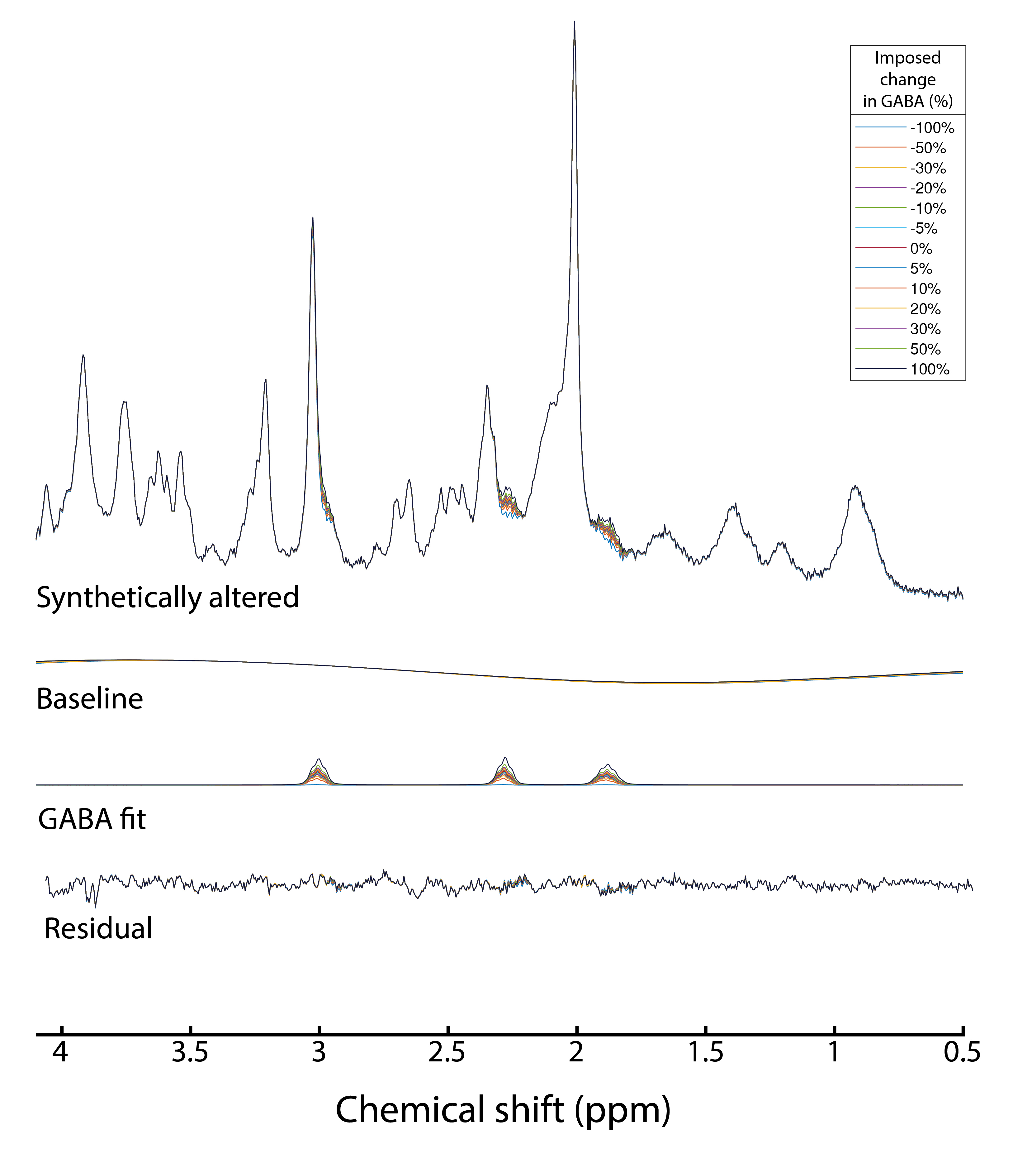
Synthetically altered spectra were generated by adding synthetic GABA signal to the main test spectra⁸. The simulated GABA spectrum was first normalized to match the amplitude and linewidth of the LCModel-fitted GABA resonance in each main test subject. The synthetic GABA signal intensity varied over the range: 0%, ±5%, ±10%, ±20%, ±30%, ±50%, ±100% (figure 1).
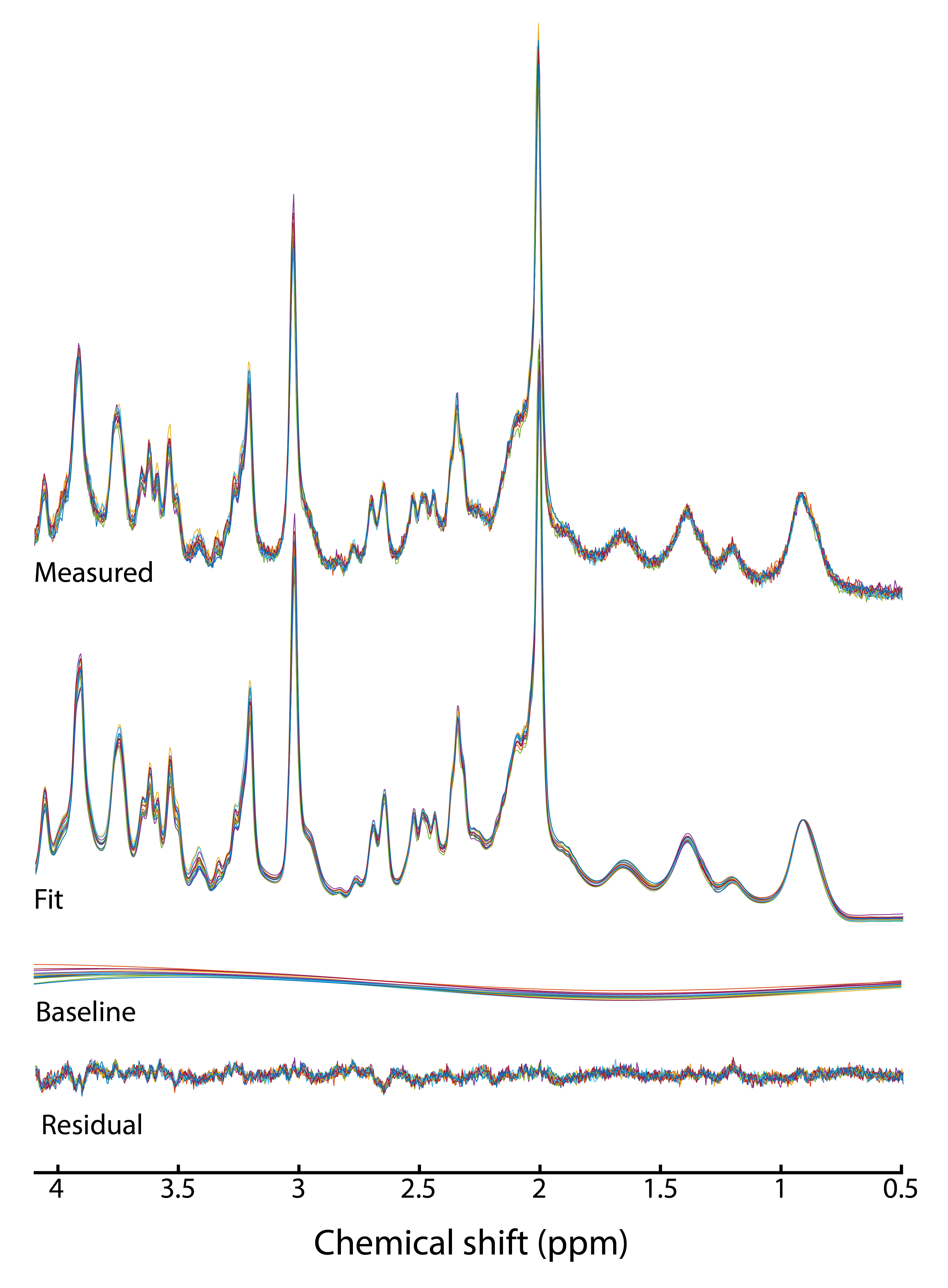
Analysis: The ability to quantify GABA by LCModel over the range of the imposed changes was evaluated using five approaches (table 1) combining LCModel parameters associated with: 1) macromolecules (MM) – measured MM (NSIMUL=6 to enable the simulation of potential lipid signals between 1 and 2 ppm) and simulated MM (NSIMUL=11); 2) baseline flatness controlled by the node spacing of the spline function – flexible (DKNTMN=0.15) and stiff (DKNTMN=5) baseline; 3) soft concentration concentrations – none (NRATIO=0) and [GABA]/([tNAA]+[tCr]+[tCho])=0.04±0.04 (NRATIO=13).
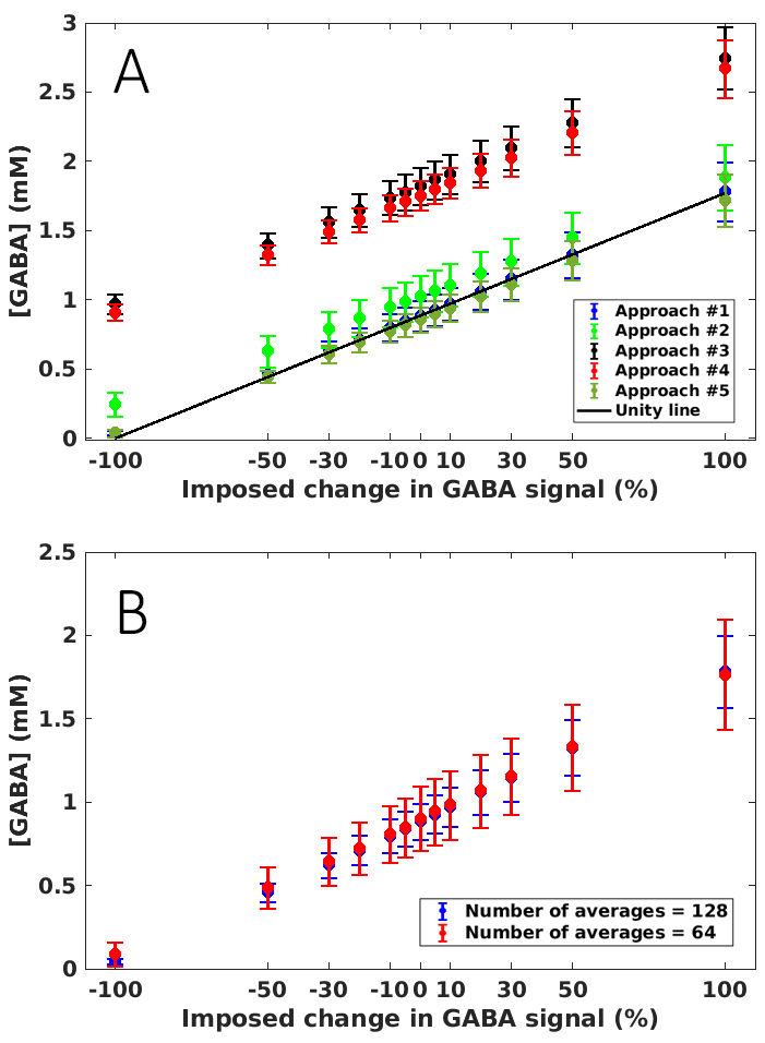
The regression line of the imposed change vs. [GABA] for each approach was compared with the unity line.
Influence of SNR on GABA quantification was studied by using half of the total averages (64) over the range of the imposed changes.
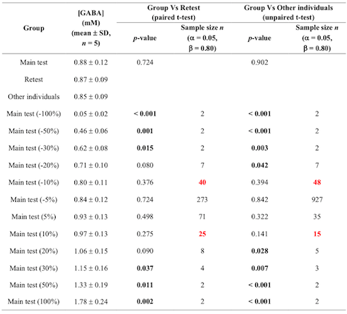
Power calculation was used to evaluate the sensitivity to detect differences in GABA levels in the test-retest group (paired t-test) and the other individuals (unpaired t-test).

Results and discussion

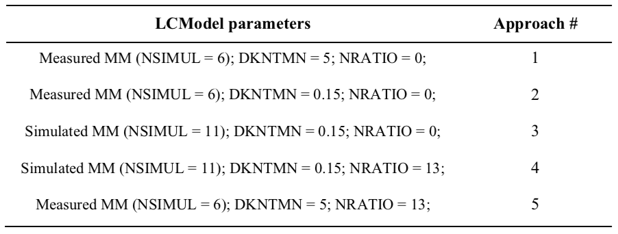
Data were of excellent quality with SNR (signal intensity at 2.01 ppm to noise: [-1.00,-2.00] ppm) = 189±22 and the linewidth (tCr peak at 3.03 ppm) = 8.1±0.3 Hz for the entire dataset (n=15), (figure 2).
LCModel fits were of high quality with no structured signals left in the residual in any of the five approaches. The regression line fitted through the GABA concentrations for the approach #1 was the closest to the unity line (R²=0.99) (figure 3A). Imposing a stiff baseline in presence of experimental MM (approach #1 and #5: R²=0.99) better approximated the unity line than a flexible baseline (approach #2: R²=0.86). The flexibility in the baseline introduces an overestimation in [GABA] that is larger as the imposed change decreases.
Using simulated MM, intercepts of the approach #3 and #4 were 106% and 98% higher than the intercept of approach #1, which might be due to a severe underestimation of macromolecules contribution to the signal around GABA resonances.
Imposing concentration ratio priors and measured MM (approach #5) resulted in an underestimation in [GABA] of ~3% over the imposed change with respect to [GABA] evaluated with the approach #1. With the current setting of priors, the underestimation is relatively small but care needs to be taken when using prior information in data in which [tNAA], [tCr] and [tCho] are changed.
Influence of SNR: When using half of the total averaged and the approach #1, the regression line was still close to the unity line (R²=0.99), but the SDs increased 2- and 3- fold with respect to the 128 averages (figure 3B). Decreasing the acquisition time does not influence the mean value of [GABA] in a cohort but the SD.
Power calculation: Significant differences in approach #1 were observed between ±30% imposed change and the retest group, and between ±20% imposed change and the other individuals. ±10% imposed change could be detected with n=25 and 40, respectively, with respect to the retest group, and with n=15 and 48 with respect to the other individuals (table 2).

Conclusions

This study evaluated different strategies to fit GABA signal with LCModel in 7-T data. The results showed that LCModel can correctly quantify GABA concentration over the imposed change using the fitting approach with measured MM, stiff baseline and no concentration ratio priors. The reduction in SNR did not influence average [GABA], but SD between subjects. The 10% group differences could be observed at 7 T with reasonable sample sizes.

Acknowledgements

Funding: This work was supported by the National Institutes of Health [grant numbers R01MH113700, R01AG039396, P41 EB015894, P30 NS076408] and the W.M. Keck Foundation.