Introduction

There have been numerous studies^1-4 of the governing SNR equations, however the majority of these scaling laws do not fully capture effects of sequence timing, tissue properties and other parameters. This may result in significant deviations of actual SNR scaling from theory. Accordingly, the objective of the present work is to investigate and represent SNR scaling as a function of static field.

Methods

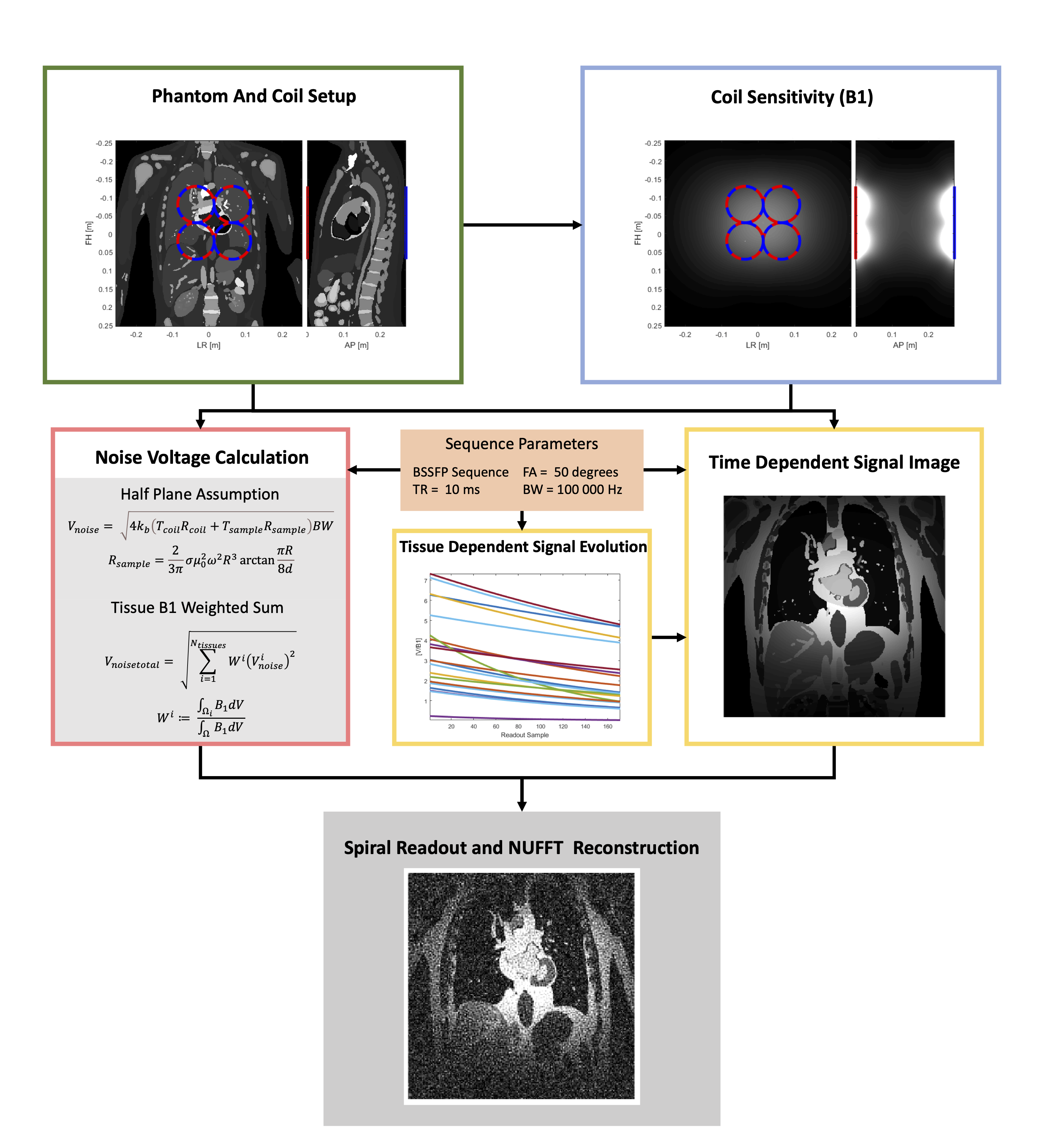
To capture field dependent SNR changes, first-principle simulation code was implemented to generate images at varying field strengths. The simulation allows the user to define various imaging parameters to generate synthetic images. If the parameters are not physically possible, they are automatically adjusted. Additionally, the simulation adjusts sequence timing (acquisition time), in order to comply with specific absorption rate (SAR) limits and to satisfy bandwidth criteria. A simplified flowchart is given in Figure 1.

Generated images are based on the XCAT⁵ phantom, which is expanded with field dependent tissue properties including T1, T2, T2* and conductivity. The phantom provides realistic anatomy and permits tissue- and organ-dependent noise source calculations.
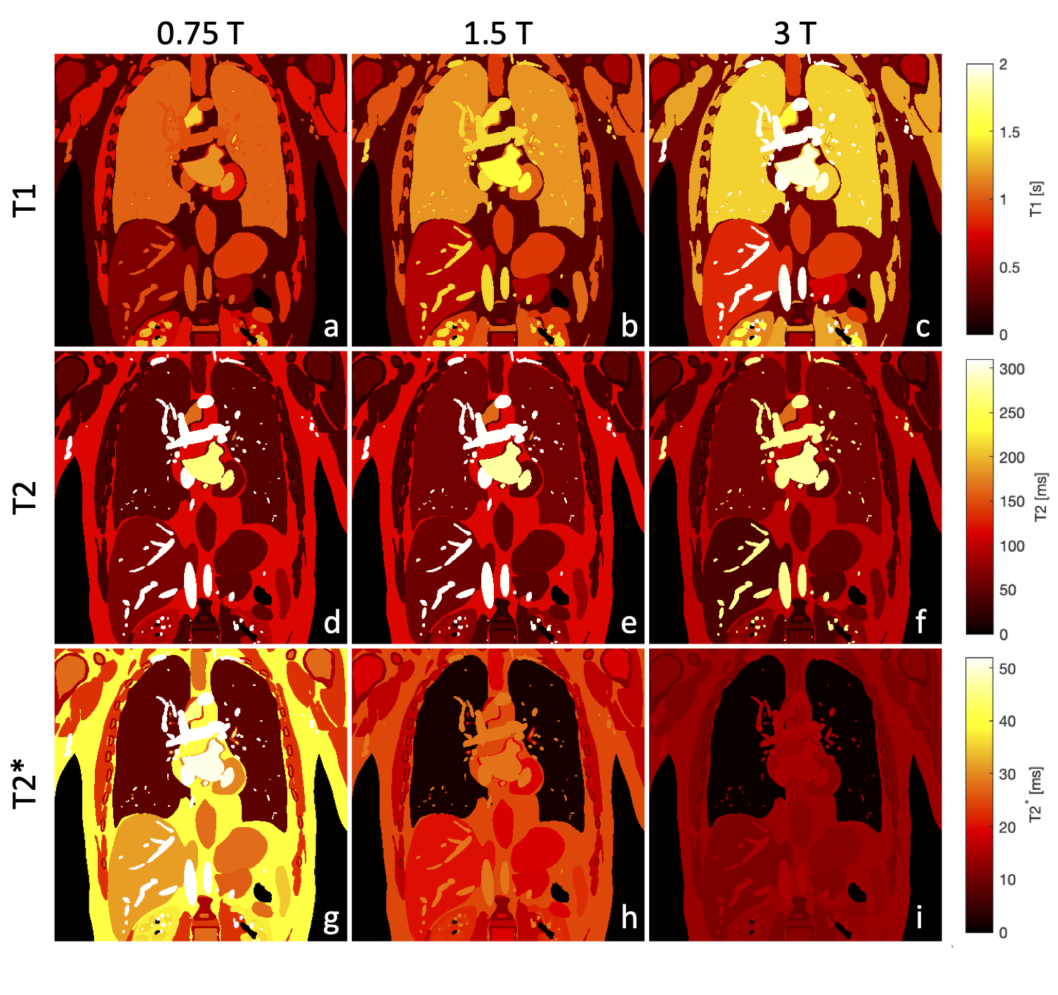
Tissue properties are taken from the ITIS database⁶, with lung data taken from other literature^7-8. T1 values are fit using the method from Bottomley⁹, while T2 values are fit linearly. T2* is calculated as follows for all tissues except lung parenchyma, for which data is used,$$T_2^*=\frac{1}{\frac{1}{T_2}+\frac{\gamma}{2\pi}\delta{}B_0}$$where $$$\delta{}B_0$$$ is field inhomogeneity and $$$\gamma$$$ is the gyromagnetic ratio. Figure 2 compares the relaxation properties at 0.75, 1.5 and 3T.

For the examples shown, signal was calculated using the balanced SSFP signal¹⁰. The overall noise contribution is calculated following the definition by Darrasse⁴, where sample resistance is estimated by assuming an infinite, homogeneous half-plane, which can be simplified to$$V_{noise}=\sqrt{4k_b(T_{coil}R_{coil}+T_{sample}R_{sample})BW}$$ $$R_{coil}\propto\sqrt{B_0}\quad\quad R_{sample}\propto{}B_0^2$$where $$$BW$$$ is bandwidth, $$$T$$$ is temperature and $$$R$$$ is resistance.
If the $$$B_0$$$ scaling for signal and noise are combined, while ignoring relaxation, one obtains two possible SNR scaling laws, $$$SNR\propto{}B_0^{7/4}$$$ for coil dominated and $$$SNR\propto{}B_0$$$ for sample dominated noise, in agreement with literature^1-4.
In order to better represent the noise contribution, each tissue has its half-plane noise calculated, and all tissue noise values are combined in a weighted sum where weighting is based on the receiver coil $$$B_1$$$ sensitivity at each tissue. Accordingly, tissues that have larger $$$B_1$$$ sensitivity contribute more to the total induced noise. This is expressed as$$ V_{noisetotal}=\sqrt{\sum_{i=1}^{N_{tissues}} W^i(V_{noise}^i)^2}\quad\quad W^i:=\frac{\int_{\Omega_i}B_1dV}{\int_{\Omega}B_1dV}$$where $$$W^i$$$ and $$$\Omega_i$$$ are the weighting factor and integration volume of tissue $$$i$$$, respectively.

When adjusting sequence timings, SAR plays a key role. Changes in field strength result in significant changes in SAR, as $$$SAR\propto{}B_0^2$$$. This can be exploited to achieve shorter RF pulses and subsequently longer acquisition time.
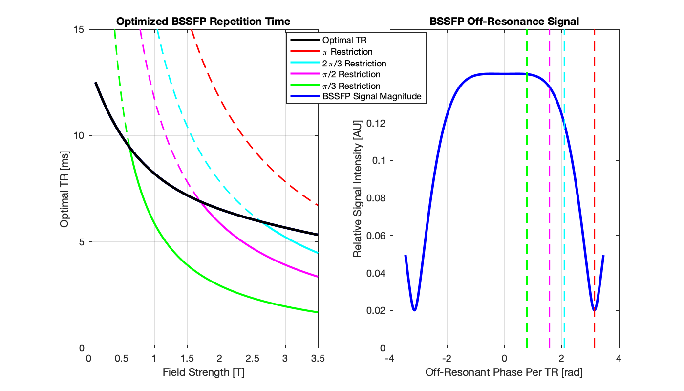
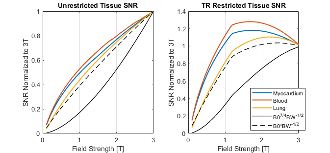
In addition to image generation, the same theory and method were employed to determine the optimal sequence parameters, maximizing SNR normalized by repetition time (division by root of repetition time). Results thereof can be seen in Figures 4 and 5.

Images were simulated using a spiral readout. Realistic spiral trajectory generation were based on Pipe¹¹. Images were reconstructed using NUFFT¹².
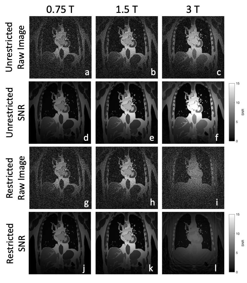
All images were generated with a FOV of 400x400mm, resolution of 2x2mm² and slice thickness of 1cm. Field inhomogeneity was set to 0.5ppm at all field strengths, and gradient limits were 40mT/m strength and 200T/m/s slew rate. A set of generated images and SNR maps is shown in Figure 3.

Results and Discussion

In the general unrestricted cases (Figure 3a-e), as field strength increases, there is a corresponding increase in image SNR. It is worth noting that this increase is less than linear with field, which is the scaling for the sample noise dominated regime. More interestingly is the case where repetition time restriction is incorporated (Figure 3g-l).

If balanced SSFP dark bands are shifted by restricting the repetition time such that phase accumulation over each repetition is limited, the relations as shown in Figure 4 are obtained. The effect can be clearly seen in Figure 3g-l, where there is a significant decrease in the SNR at 3T when the off-resonance phase is restricted. In addition to a decrease in the SNR, there is a decrease in tissue contrast at 3T due to the need to use lower flip angles to achieve such a short repetition time. This behaviour can be seen again in Figure 5, where the restriction causes a decrease in SNR for higher fields when compared to the unrestricted case or the SNR scaling laws.

The deviation from traditional SNR scaling laws, both in the unrestricted and restricted cases, is a strong motivator to further investigate field-dependent SNR scaling.

Conclusion

It has been demonstrated that, when tissue properties and SAR dependencies are taken into account, scaling of SNR with field strength can deviate significantly from commonly used equations. This is specifically interesting for the case of lower field systems, as these changes tend to benefit lower field strengths, making them more appealing in comparison to traditional high field systems.

Acknowledgements

The work was funded in parts by EU Horizon 2020 FETFLAG MetaboliQs.