2176
Learned Proximal Convolutional Neural Network for Susceptibility Tensor Imaging1Department of Biomedical Engineering, Johns Hopkins University, Baltimore, MD, United States, 2F.M. Kirby Research Center for Functional Brain Imaging, Kennedy Krieger Institute, Baltimore, MD, United States, 3Department of Radiology and Radiological Sciences, Johns Hopkins University, Baltimore, MD, United States
Synopsis
We extended a Learned Proximal Convolutional-Neural-Network (LP-CNN) model used in scalar-based Quantitative Susceptibility Mapping (QSM) to tensor-based Susceptibility Tensor Imaging (STI). To improve the accuracy in reconstructed susceptibility anisotropy and tensor eigenvectors, we devised a decomposition loss function to balance training errors in isotropic and anisotropic components. Results using a synthetic dataset demonstrated that, compared to the conventional iterative approach, LP-CNN-STI provides better estimates of susceptibility tensor and smaller errors in anisotropy and eigenvectors. This deep learning-based STI method naturally incorporates the STI physical model, and is a first step toward development of learning-based STI potentially with less acquisition orientations.
Introduction
Susceptibility Tensor Imaging (STI) is a recent MRI technique that estimates and quantifies anisotropic tissue magnetic susceptibility from multiple gradient echo (GRE) imaging phases1. Compared to Quantitative Susceptibility Mapping (QSM), which assumes isotropic tissue magnetic susceptibility2,3, STI utilizes symmetric rank-2 tensors to characterize tissues with highly organized microstructure that exhibit macroscopic susceptibility anisotropy1,4. Similar to Diffusion Tensor Imaging (DTI), the reconstructed susceptibility tensor in STI can be used to reveal brain tissue microstructure such as white matter fiber pathways4. However, due to the requirement of acquiring MR phase at multiple orientations and the ill-posed inverse problem, in vivo STI and STI-based fiber tracking is still very challenging, even with the use of regularization5.Recently, deep learning has shown great promise in solving various imaging inverse problems with fast and high-quality reconstruction6,7. Learned Proximal Convolutional Neural Network (LP-CNN) is a physics-informed deep learning approach that has been applied in multi-orientation QSM8. This approach solves the QSM dipole inversion problem with separated data-driven restoration priors and physical model-aware iterative solvers. Here, we extend the scalar-based LP-CNN to a tensor-based LP-CNN for STI reconstruction by incorporating the more complex STI forward operator. Moreover, to improve reconstruction accuracy for mean magnetic susceptibility (MMS), magnetic susceptibility anisotropy (MSA) and Principal Eigenvector (PEV), we introduce a decomposition loss that factorizes the susceptibility tensor into its isotropic and anisotropic parts, helping balance the training losses on both components. Testing on synthetic data shows that the LP-CNN-STI achieved slightly improved results compared to the conventional STI solution using iterative LSQR solver.
Methods
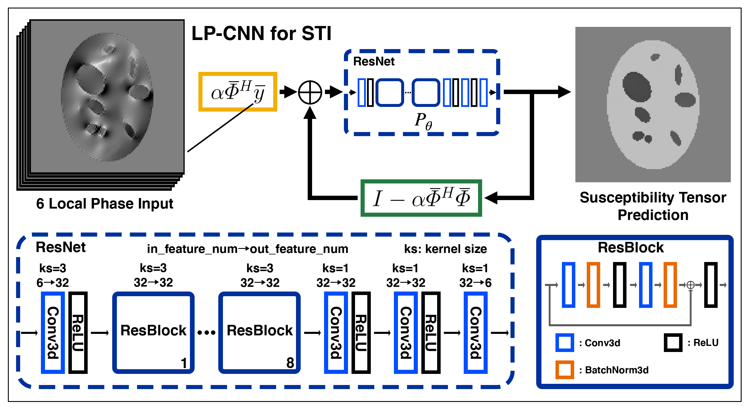
For model training and testing, we synthesized 16 phantoms (image size $$$128\times128\times128$$$ voxels), each containing 32 oval shape components at randomly selected locations with random orientations. Each component is piecewise homogeneous and has either isotropic or anisotropic susceptibility. Two types of isotropic susceptibility values, i.e. ~0.05ppm (cortical gray matter) or ~0.25ppm (iron rich nuclei) are randomly assigned to 25% of components, while anisotropic susceptibility with about -0.03ppm MMS and 0.02ppm MSA (simulating white matter) are randomly assigned to the other 75%. We then generated 20 phase measurements according to the STI forward model at random orientations evenly distributed over a sphere for each phantom without adding noise. We randomly chose 6 of the 20 simulated phases and the underlying susceptibility tensor to form a data pair in the dataset. Twelve phantoms were used for training and four phantoms for validation. The LP-CNN model used for STI training was extended from LP-CNN for QSM8. LP-CNN contains a gradient descent step and a proximal regularization step in each iteration. We modified the forward operator in the gradient descent step and adjusted the proximal regularizer neural network to fit 6-channel symmetric susceptibility tensor, resulting in the update:$$\hat{x}_{i+1}=P_\theta \left(\alpha\bar\Phi^H \bar y + \left(I -\alpha\bar\Phi^H \bar\Phi\right)\hat{x}_i\right)$$where $$$\bar y$$$ and $$$\bar\Phi$$$ are concatenated phase and STI forward operator. Through tensor decomposition $$$T=\frac{1}{3}trace(T)I+(T-\frac{1}{3}trace(T)I)=T_{iso}+T_{aniso},$$$ we also employ a decomposition loss function by calculating a reconstruction error on the isotropic and anisotropic components of the tensors separately with different weighting. The overall LP-CNN model design is in Figure 1. We trained our LP-CNN with decomposition loss and Adam optimizer using 3D patch data with a size of $$$64\times64\times64$$$ voxels. The total training time was approximately one week. We compared the results to LP-CNN training with L1-norm loss only and the conventional iterative STI employing LSQR9 solver (tolerance of 1e-4 and max iteration of 100, with only regularization to constrain the STI solution inside a brain mask) on the validation set.Results
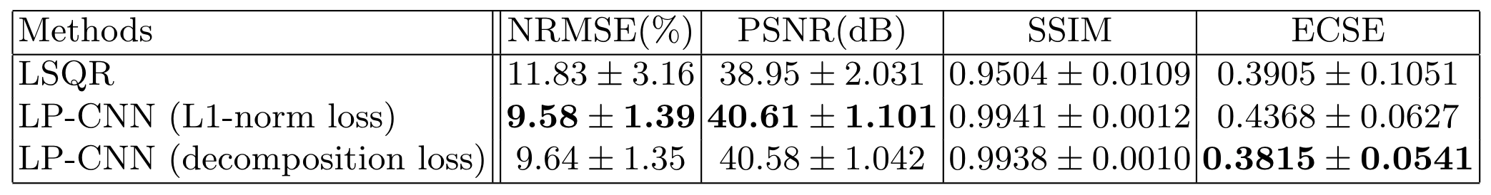
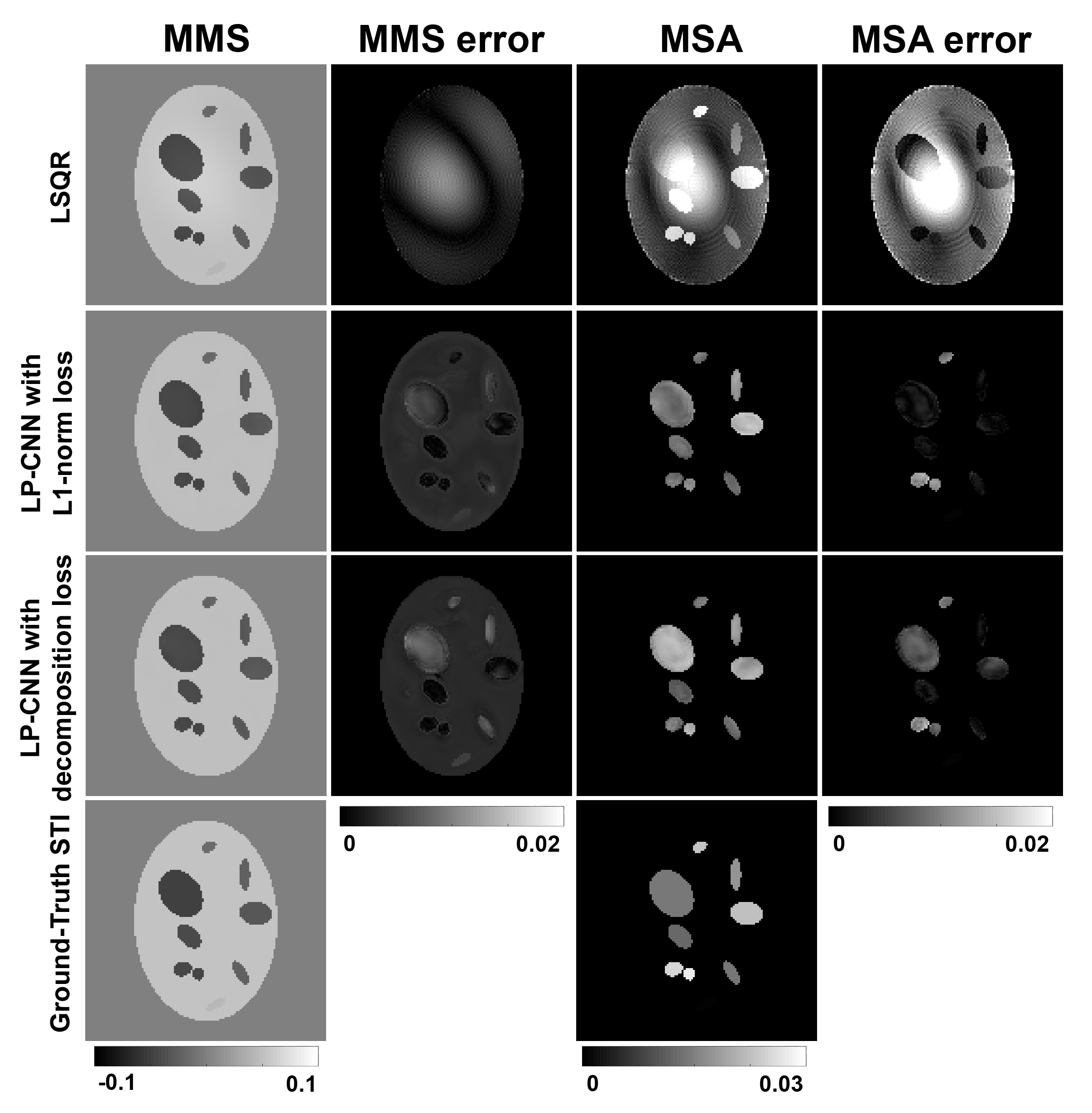
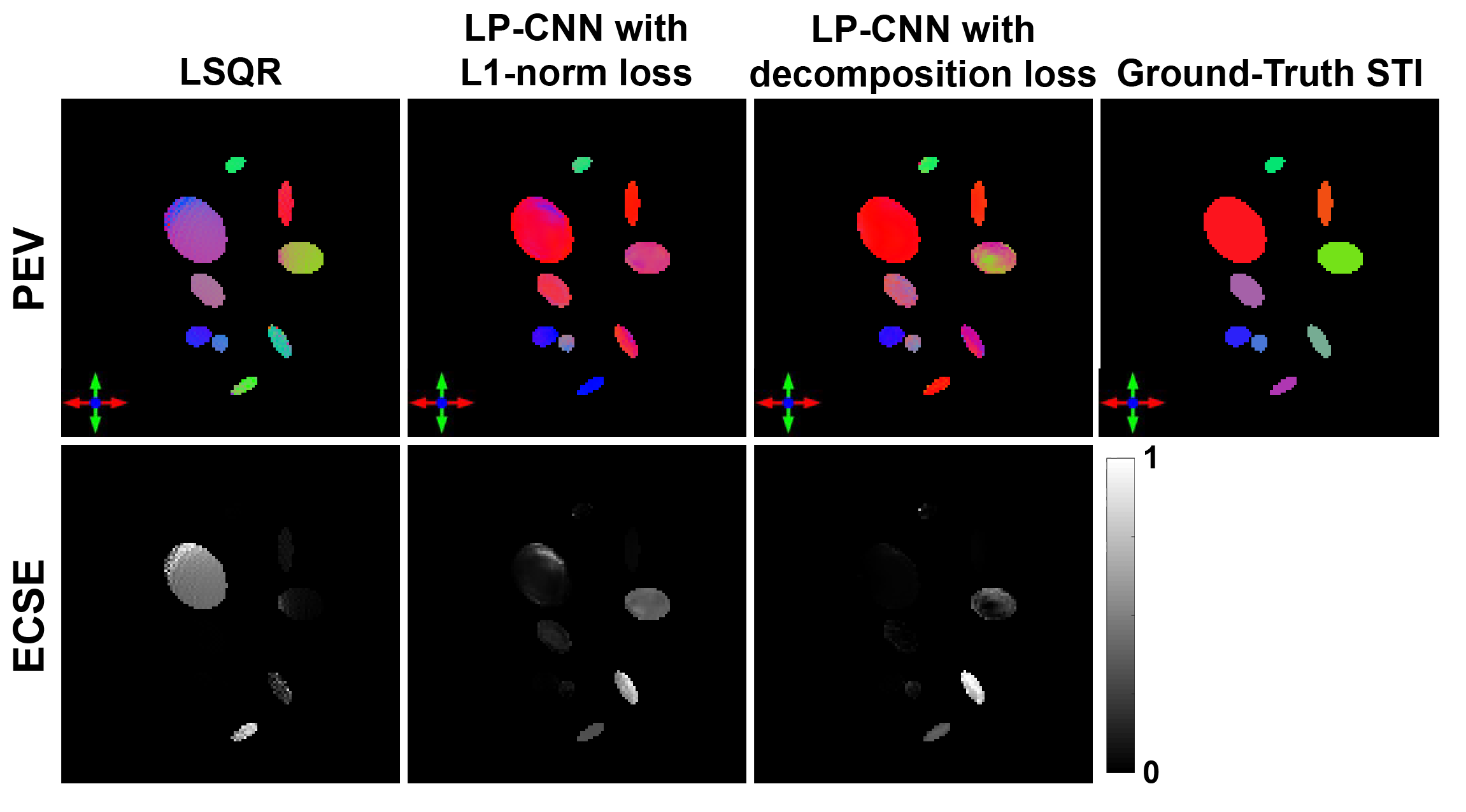
Table 1 summarizes the STI reconstruction results on the validation set using different methods. The Eigenvector Cosine Similarity Error (ECSE) measures the PEV dissimilarity in anisotropic regions where $$$ECSE=1-|\langle PEV_1,PEV_2\rangle|.$$$ The result shows that LP-CNN with decomposition loss achieves a PSNR of 40.58±1.04 dB and an ECSE of 0.38±0.05, which surpasses the LSQR solution. Figure 2 displays the reconstructed MMS and MSA maps from one validation example and their corresponding error maps compared to ground-truth. LP-CNN has less artifacts compared to LSQR, especially in MSA. Figure 3 displays the color-coded maps of the reconstructed principal susceptibility eigenvector (corresponds to the largest or least negative eigenvalue) and the ECSE maps. Both LP-CNN and LSQR have relatively low reconstruction error in the anisotropic areas, but different error patterns are observed.Discussion
Our decomposition loss separates isotropic and anisotropic regression components during training and is flexible in weighing isotropic and anisotropic parts independently, providing a better optimization strategy for STI. Compared to the LSQR method, LP-CNN not only reconstructs STI with less artifacts and smaller orientation errors but also executes faster (~500s versus ~10s). The present work only demonstrates the feasibility of deep-learning based STI with ideal noise-free phase measurements acquired at 6 orientations with large rotation angles. Future investigations need to test the LP-CNN based STI with different numbers of phase measurements at different noise levels and rotation angles.Conclusion
We proposed a LP-CNN model for STI reconstruction, and demonstrated its capability of reconstructing MMS, MSA and PEV in synthetic phantoms. This is the first deep learning-based STI method incorporating physical model forward operators using synthetic phantoms, and is a first step towards development of deep-learning based STI reconstruction.Acknowledgements
This work was supported by NCRR and NIBIB (P41EB015909) of the National Institutes of Health.References
1Chunlei Liu. Susceptibility tensor imaging. Magnetic Resonance in Medicine: An Official Journal of the International Society for Magnetic Resonance in Medicine 63(6), 1471–1477, 2010.
2Yi Wang and Tian Liu. Quantitative susceptibility mapping (qsm): decoding mri data for a tissue magnetic biomarker. Magnetic resonance in medicine, 73(1):82–101, 2015.
3Chunlei Liu, Wei Li, Karen A Tong, Kristen W Yeom, and Samuel Kuzminski. Susceptibility-weighted imaging and quantitative susceptibility mapping in the brain. Journal of magnetic resonance imaging, 42(1):23–41, 2015.
4Wei Li, Chunlei Liu, Timothy Q Duong, Peter CM van Zijl, and Xu Li. Susceptibility tensor imaging (sti) of the brain. NMR in Biomedicine, 30(4): e3540, 2017.
5Xu Li, Peter van Zijl. Mean magnetic susceptibility regularized susceptibility tensor imaging (mmsr-sti) for estimating orientations of white matter fibers in human brain. Magnetic resonance in medicine 72(3), 610–619, 2014.
6Jaeyeon Yoon, Enhao Gong, Itthi Chatnuntawech, Berkin Bilgic, Jingu Lee, Woojin Jung, Jingyu Ko, Hosan Jung, Kawin Setsompop, Greg Zaharchuk, et al. Quantitative susceptibility mapping using deep neural network: Qsmnet. NeuroImage, 179:199–206, 2018.
7Olaf Ronneberger, Philipp Fischer, Thomas Brox. U-net: Convolutional networks for biomedical image segmentation. International Conference on Medical image computing and computer-assisted intervention. pp. 234–241. Springer 2015.
8Kuo-Wei Lai, Manisha Aggarwal, Peter van Zijl, Xu Li, Jeremias Sulam. Learned proximal networks for quantitative susceptibility mapping. International Conference on Medical Image Computing and Computer-Assisted Intervention. pp. 125–135. Springer 2020.
9Christopher C Paige, Michael Saunders. LSQR: An algorithm for sparse linear equations and sparse least squares. ACM Transactions on Mathematical Software (TOMS) 8.1 (1982): 43-71.
Figures