2163
Global and Local Deep Dictionary Learning Network for Accelerating the Quantification of Myelin Water Content1School of Biomedical Engineering, Shanghai Jiao Tong University, Shanghai, China
Synopsis
Acceleration of the myelin water fraction (MWF) mapping at R=6 using a Global and Local Deep Dictionary Learning Network (GLDDL) is demonstrated in this study. The global and the local spatiotemporal correlations in the relaxations are learned simultaneously. The global temporal encode-decoder layers are utilized to reduce the computational complexity of the local DL network and improve the denoising performance. The deep DL network utilizes the merits of traditional DL and deep learning to improve the reconstruction. The high-quality MWF maps obtained from the GLDDL network has demonstrated the feasibility to accelerate the whole brain MWF mapping in 1 minute.
Introduction
Acceleration for the T2/T2* relaxation based MWF mapping has been achieved using parallel imaging and compressed sensing at a reduction factor (R) of 21,2. Dictionary learning (DL) has also been used to accelerate the parametric imaging by exploiting the global or local spatiotemporal correlations inside the data. In the global scheme, the dictionaries are usually used to depict the spatiotemporal features shared by all pixels3,4. In the local scheme, the dictionaries are used to capture the spatiotemporal correlations within the patches5. Deep learning network based reconstruction has been proposed recently to accelerate the parametric imaging6. The Convolutional Recurrent Neural Networks (CRNN) learns the spatiotemporal dependencies inside the CEST data and recovers the high-quality images from the undersampled data7. In this study, a Global and Local Deep Dictionary Learning Network (GLDDL) is proposed to explore the global and local spatiotemporal correlations jointly. The deep DL network jointly utilizes the merits of traditional dictionary learning and deep learning to improve the performance of MRI reconstruction. The GLDDL network is applied to accelerate the quantification of myelin water content.Theory
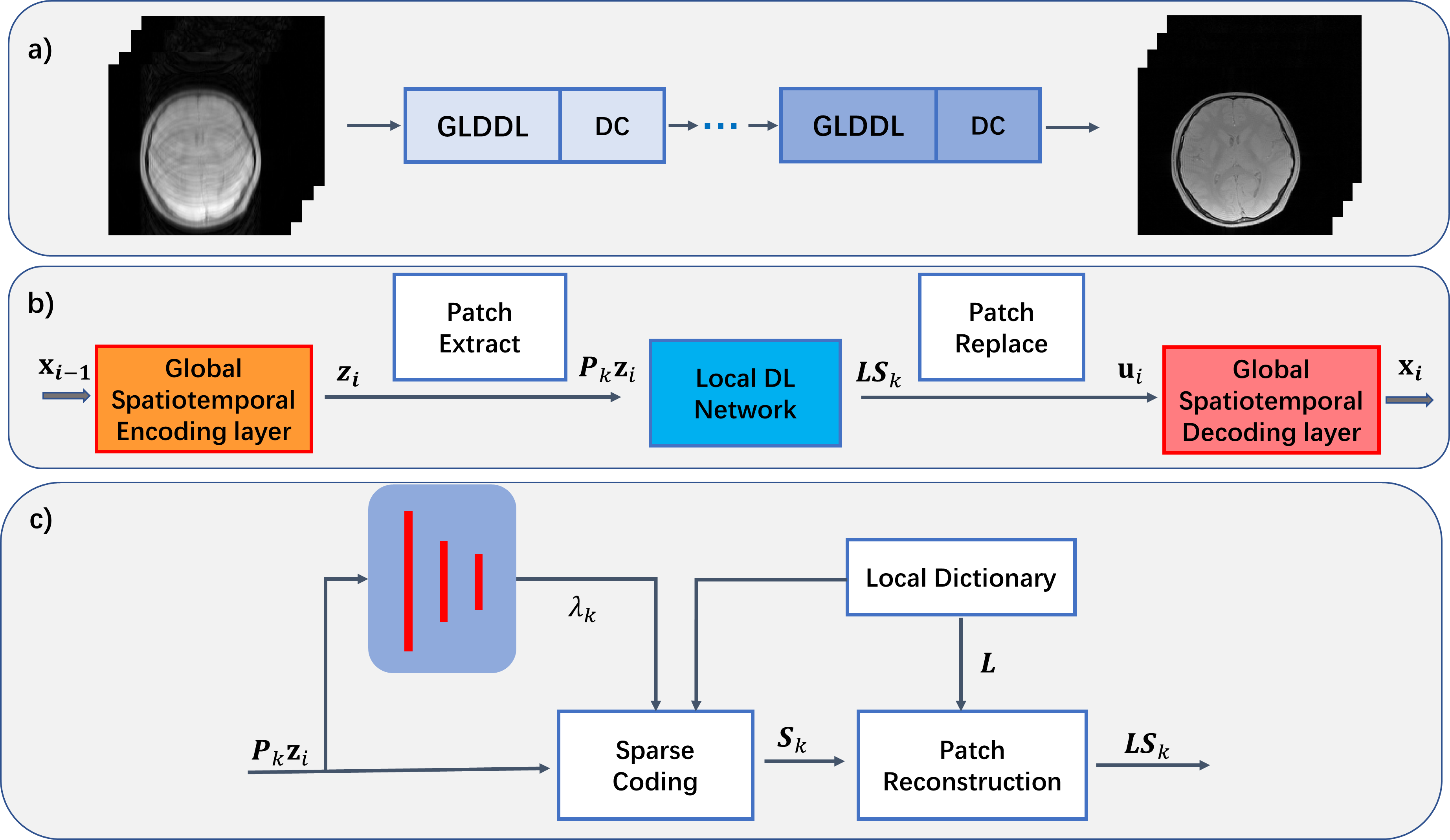
The GLDDL network learns both global and local spatiotemporal correlations. As shown in Figure 1, the DL network and the data consistency network are combined as a single unit. Multiple units have been concatenated together to improve the performance. The T2*WIs are first encoded by a global spatiotemporal encoder layer to reduce the temporary dimension. A patch-based local DL network is utilized to denoise the reduced datasets. The local DL network provides a dictionary to depict the characteristics of the signals and sparsely codes the linear combination of basis functions8. The denoised data are decoded by a global spatiotemporal decoder layer to obtain the T2*WIs before the data consistency (DC) layer.The GLDDL block and DC layer in the i-th unit are defined as follow:$$\underset{x}{min}\rho\left\|F_usx_i-y \right\|_2+GLDDL(x_i)$$
where $$$x$$$ is the desired images, $$$y$$$ is the undersampled k-space data, $$$s$$$ is the coil sensitivity, and $$$F_u$$$ is the undersampled Fourier operator. Firstly, a reduced dataset $$$z_i$$$ can be obtained by the global spatiotemporal encoder layer:$$z_i=Encoder(x_{i-1}).$$
Then, the local DL network is used for removing the artifacts and noise:
$$\underset{L,s_k,\lambda_k}{min}\left\|LS_k-P_kZ_i \right\|_2+\lambda_k\left\|S_k \right\|_1,$$
where $$$P_k$$$ is the patch operator to extract the k-th patch. $$$L$$$, $$$S_k$$$ are the local dictionary and the sparse coefficients, respectively. $$$\lambda_k$$$ is a regularization coefficient, which is learned through three fully connected layers. Iterative Soft Thresholding Algorithm (ISTA)9 is used to solve the sparse coding step.
The denoised dataset $$$u_i$$$ can be obtained by replacing the patches:
$$u_i=\frac{\sum_{k}P_k^T(w \bullet LS_k)}{\sum_{k}P_k^Tw}$$
where $$$w$$$ is the weighting for each pixel. The T2*WIs can be recovered by the global spatiotemporal decoder layer:
$$x_i=Decoder(u_i).$$
The encoder-decoder, the local dictionary and the $$$\lambda$$$ evaluation perceptron in the network are optimized by the end-to-end training.
Methods
Nine healthy subjects were scanned using a multi-slice mGRE sequence on a 3T MRI scanner (uMR790, United Imaging Healthcare, Ltd., Shanghai, China). Written consent was obtained before each scan. The scanning parameters were: FOV = 240×240mm2, matrix = 176×176, FA = 90°, TR = 2 s, first TE = 1.95 ms, echo spacing = 1.16 ms, echo train length = 30, slice thickness = 3 mm, 25 slices were scanned with a 1.5 mm slice gap. The whole brain scan time was 5.9 min. A variable-density random phase-encoding mask with R = 6 was used for retrospective undersampling. Datasets from 7 subjects were used for training, and the other 2 datasets were used for testing. The proposed algorithm was compared to the state-of-the-art DL with temporal gradients (DLTG)5 and the CRNN algorithms7,10. The non-negative jointly sparse (NNJS) algorithm11 was used for MWF estimation.Results
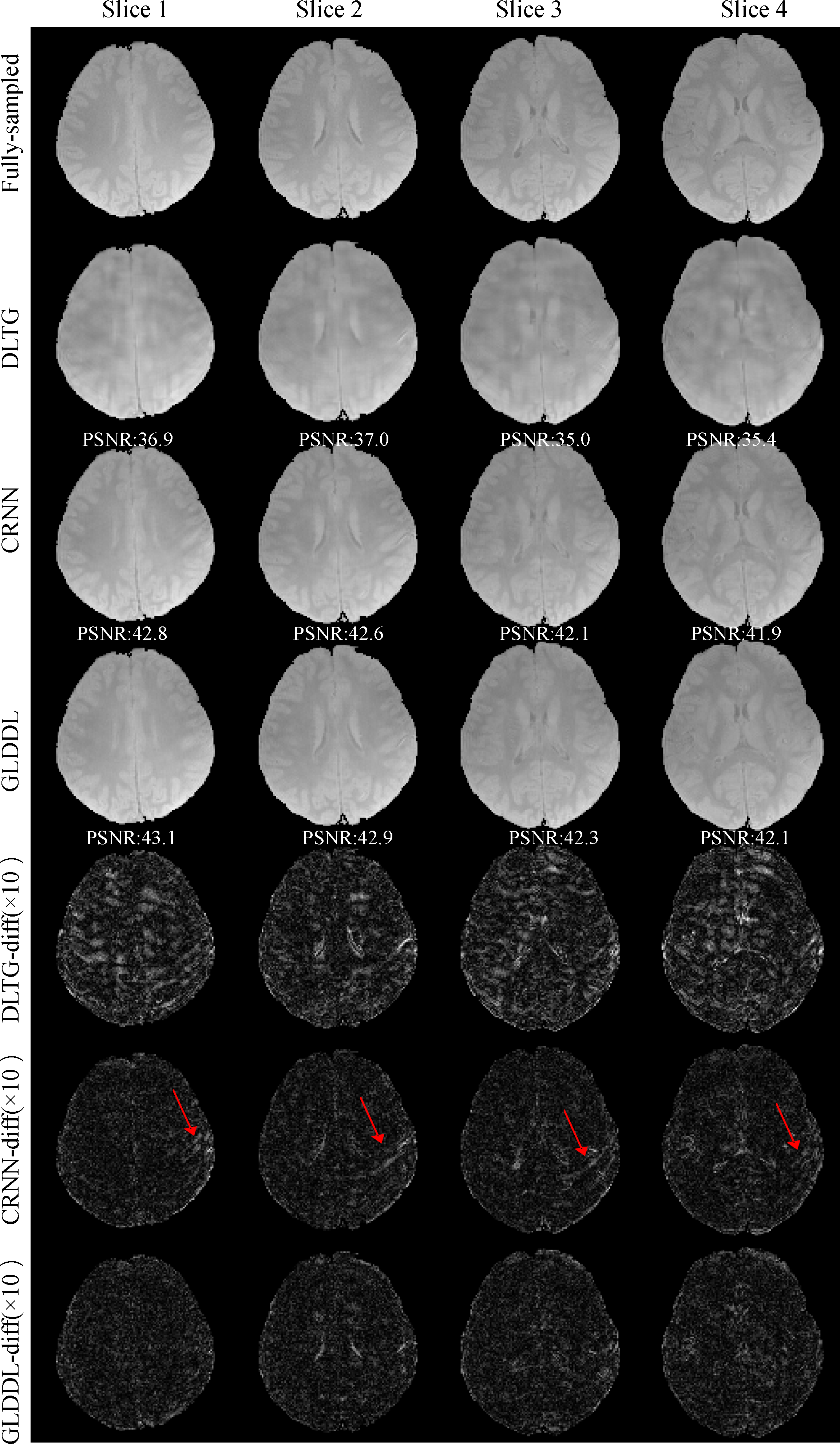
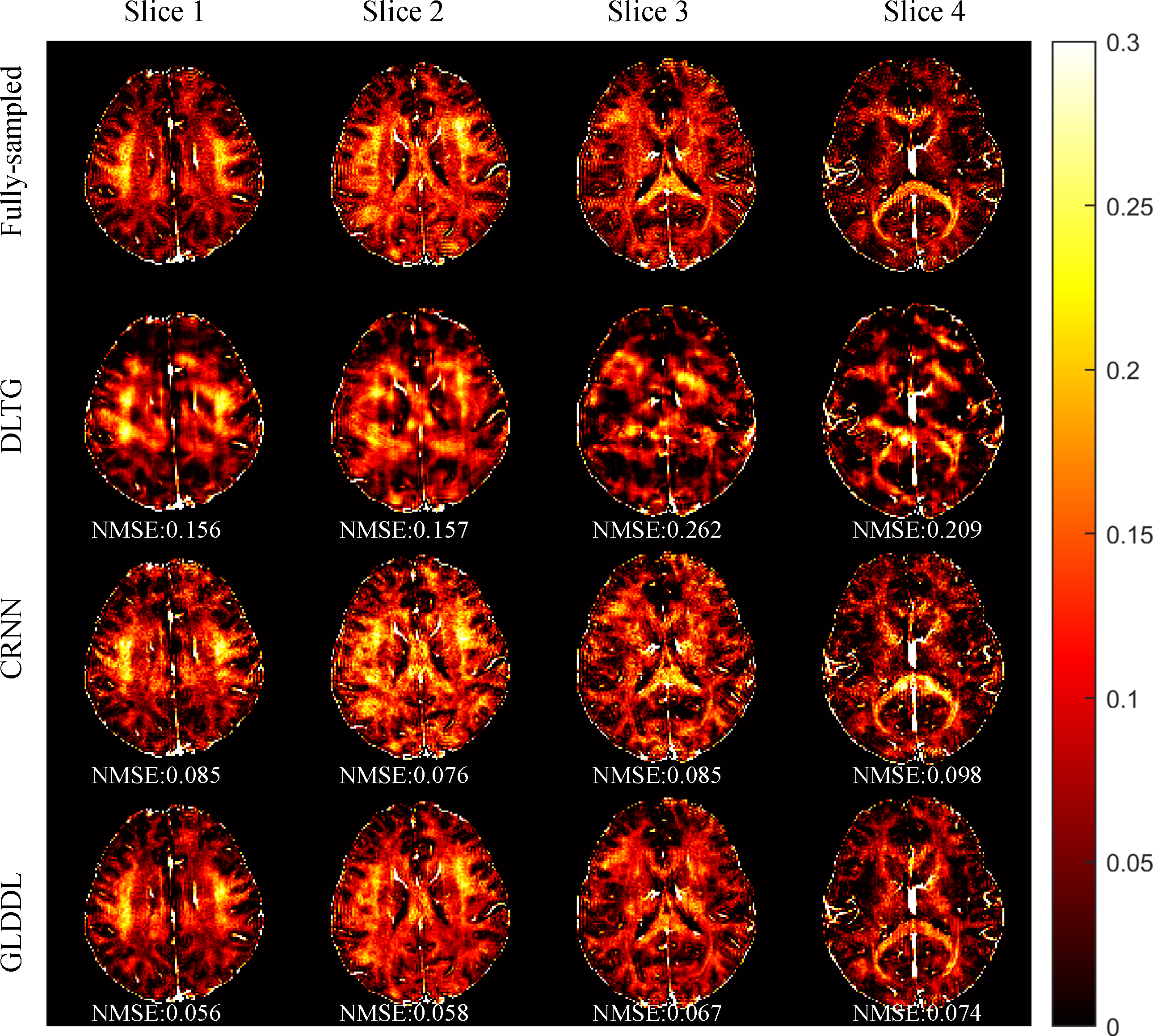
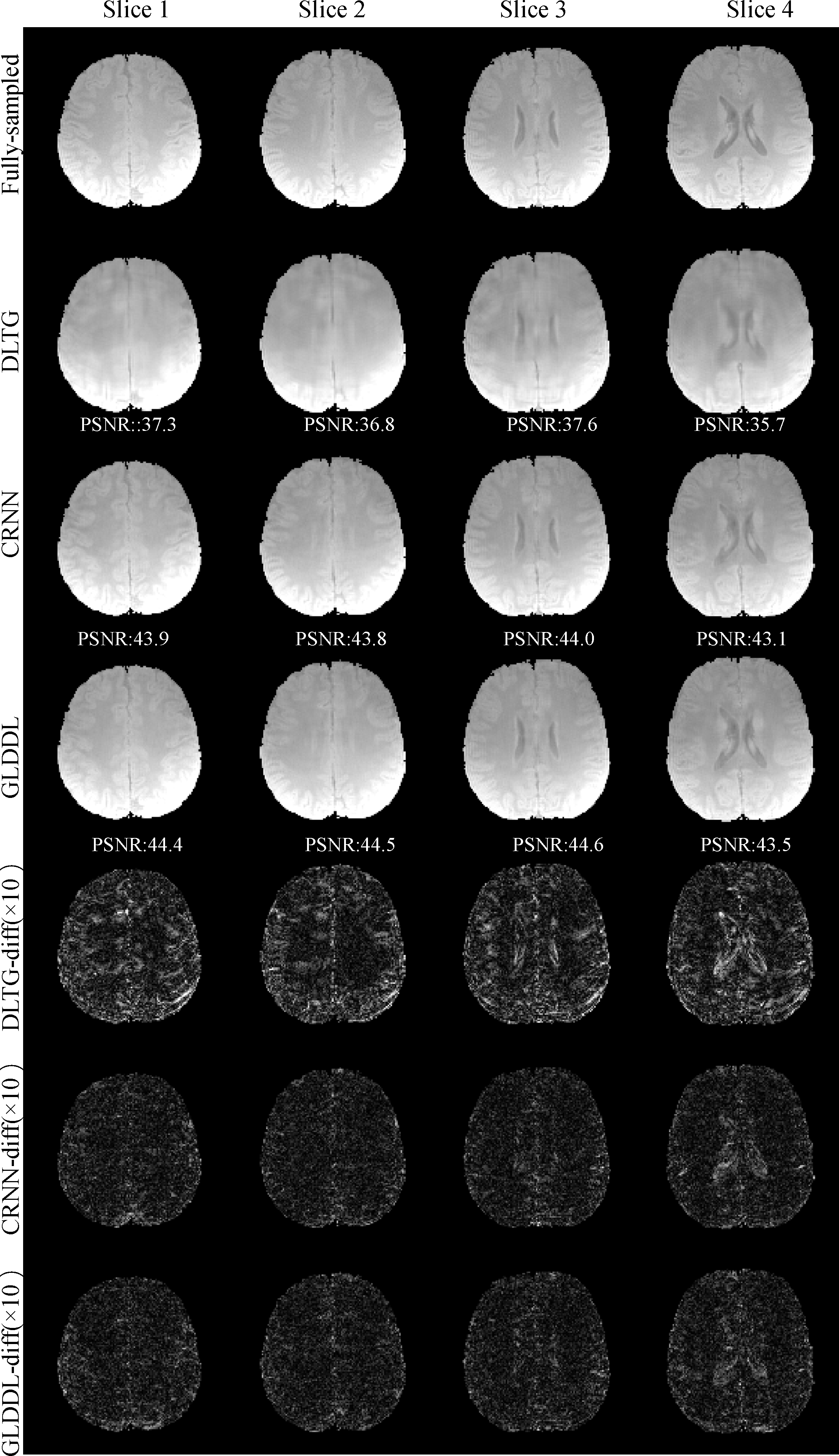
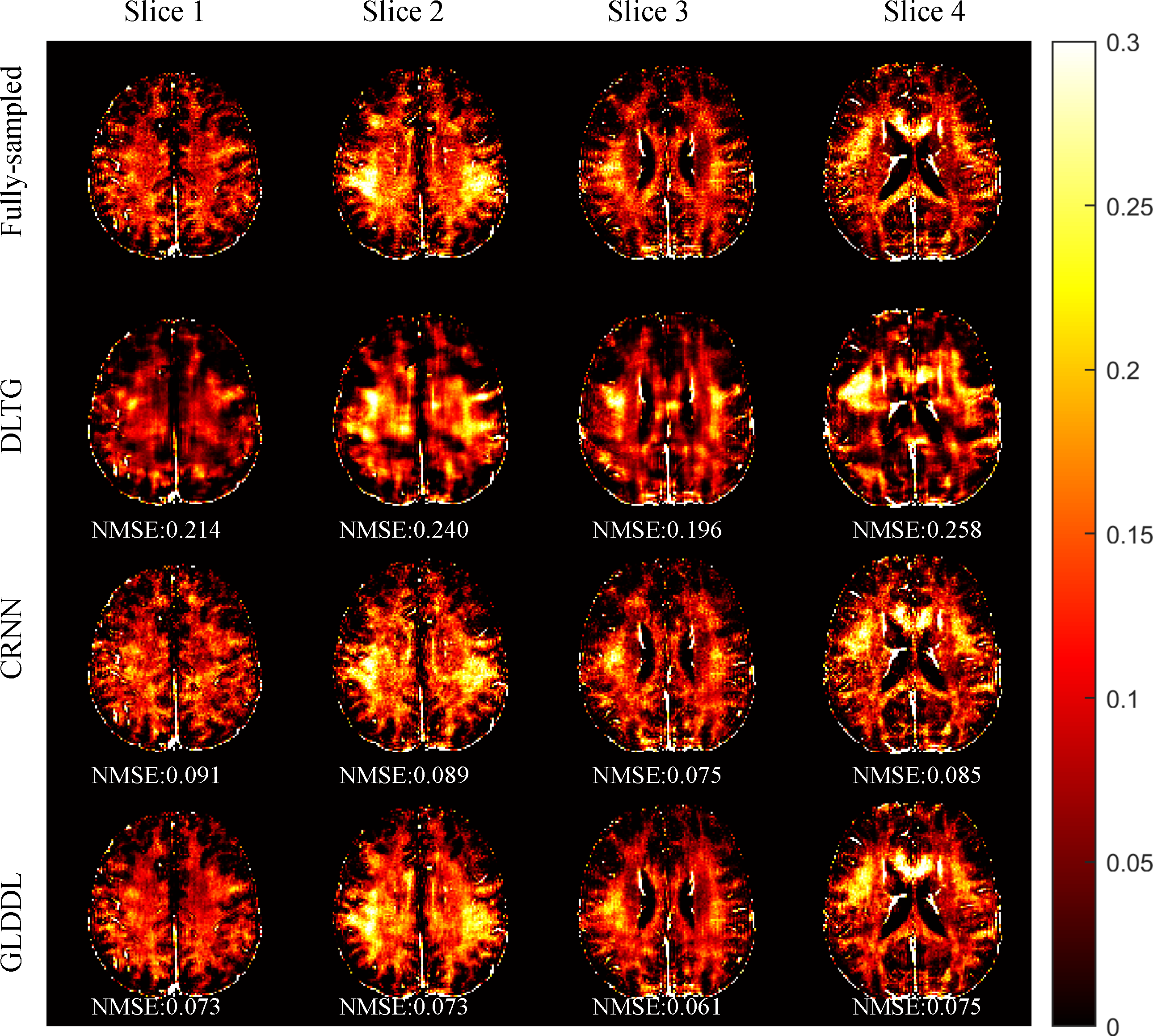
The reconstructed T2*WIs of the GLDDL network are compared to that of the DLTG and CRNN algorithms, as shown in Figure 2 and Figure 4. The T2*WIs of the GLDDL network at the first echo have minimal artifacts, while the images of the DLTG and CRNN reconstructions at the first echo obtain visible artifacts. The GLDDL network reconstructed T2*WIs of all echoes show high similarity with the fully-sampled references with the highest PSNR among the three reconstructions. The MWF maps obtained from the GLDDL network reconstruction present high quality with lower NMSE compared to the results of DLTG and CRNN, as shown in Figure 3 and Figure 5.Discussion and Conclusion
The outperformance of the proposed GLDDL network over the DLTG and CRNN reconstructions has been demonstrated by the reduced artifacts and improved similarity with the fully-sampled references in both the results of T2*WIs and MWF. The global temporal encoder-decoder layers can reduce the data size of the local DL network, and thus can improve the training speed. The GLDDL network has demonstrated the potential of accelerating MWF quantification in 1 minute with R = 6.Acknowledgements
No acknowledgement found.References
[1] Drenthen GS, Backes WH, Aldenkamp AP, Jansen JF. Applicability and reproducibility of 2D multi-slice GRASE myelin water fraction with varying acquisition acceleration. NeuroImage 2019;195:333-339.
[2] Chen H, Majumdar A, Kozlowski P. Compressed sensing CPMG with group-sparse reconstruction for myelin water imaging. Magn Reson Med 2014;71:1166-1171.
[3] Lingala SG, Jacob M. Blind compressive sensing dynamic MRI. IEEE Trans Med Imaging 2013;32:1132-1145.
[4] Bhave S, Lingala SG, Johnson CP, Magnotta VA, Jacob M. Accelerated whole-brain multi-parameter mapping using blind compressed sensing. Magn Reson Med 2016;75:1175-1186.
[5] Caballero J, Price AN, Rueckert D, Hajnal JV. Dictionary learning and time sparsity for dynamic MR data reconstruction. IEEE Trans Med Imag 2014;33:979-994.
[6] Liu F, Feng L, Kijowski R. MANTIS: Model-augmented neural network with incoherent k-space sampling for efficient MR parameter mapping. Magn Reson Med 2019;82:174-188.
[7] She H, Li B, Lenkinski R, Vinogradov E. Accelerate Parallel CEST Imaging with Dynamic Convolutional Recurrent Neural Network. In Proceedings of the 27th Annual Meeting of ISMRM, Montréal, Canada; 2019. p. 142.
[8] Scetbon M, Elad M, Milanfar P. Deep k-svd denoising. 2019;arXiv:1909.13164.
[9] Gregor K, LeCun Y. Learning fast approximations of sparse coding. In Proceedings of the 27th International Conference on Machine Learning, Haifa, Israel; 2010. p. 399-406.
[10] Qin C, Schlemper J, Caballero J, Price AN, Hajnal JV, Rueckert D. Image Reconstruction. Convolutional recurrent neural networks for dynamic MR image reconstruction. IEEE Trans Med Imaging 2019;38:280-290.
[11] Chen Q, She H, Du YP. Improved quantification of myelin water fraction using joint sparsity of T2* distribution. J Magn Reson Imaging 2020;52:146-158.
Figures