Introduction

Time resolved 3D phase contrast (4D Flow) is widely used for blood flow evaluation and visualization of flow patterns [1]. Compressed sensing (CS) method can be used to reduce the long acquisition time in 4D flow [2,3], but may under-estimate the velocity of the flow [4,5]. This underestimation can be aggravated in circumstances of turbulence [6,7], however this has not been thoroughly examined.
In this study, we examined the effect of flow estimation in the presence of turbulence in a carefully designed flow phantom experiment, which can generate both pulsatile and turbulent flow. Using the phantom we compared the effect of estimation for 4D Flow using four flow encodings and using seven encodings (also known as icosahedral flow encoding or ICOSA6).

Method

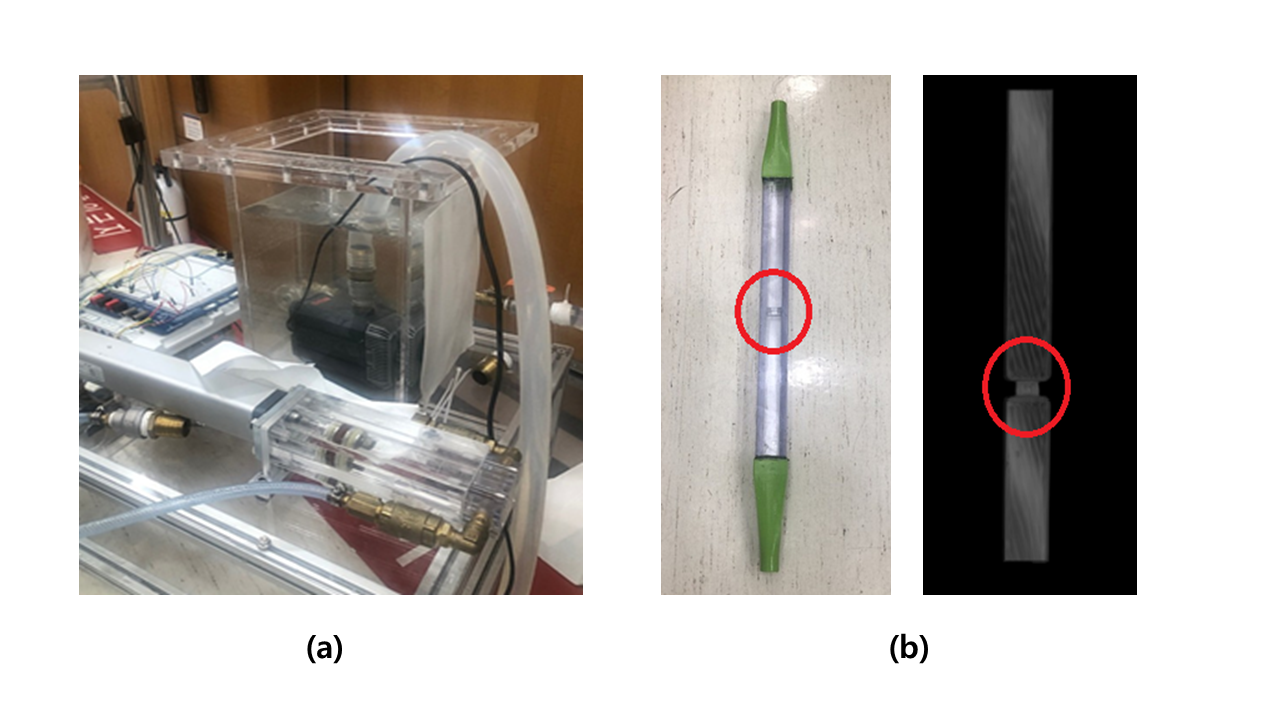
[Pulsatile jet flow phantom & Data acquisition]
Flow phantom details :
The designed and used phantom is demonstrated in Fig. 1. Turbulence was created by the contraction area located in the middle of rectangular model, which is shown in Fig.1.b. Fluid was a mixture of water and glycerol to adjust the density to 1053.8 kg/m3, and Viscosity to 3.72x10-3 kg·m-1s-1). Moreover, to increase the signal intensity, 30 mL of Contrast agent (0.5 mmol/kg, Meglumin gadoterate, Guerbet, Paris, France) was added.
Scan protocol for full acquisition :
Fully sampled data was acquired on a clinical 3 Tesla MRI scanner (Ingenia, Philips Medical Systems, Best, The Netherlands) using 32ch torso coil. Conventional 4D Flow and ICOSA6 were acquired as followed: FOV= 256x140x70mm3, spatial resolution= 2mm iso-voxel, flip angle= 10°, TR= 4.5ms, TE= 2.5ms, cardiac retrospective phase= 30, VENC= 300m/s for velocity parameter, 150m/s for turbulent estimation. In ICOSA6, one reference and six different icosahedron motion encoding with golden ratio were acquired.
[Retrospective under-sampling and Compressed sensing based reconstruction]
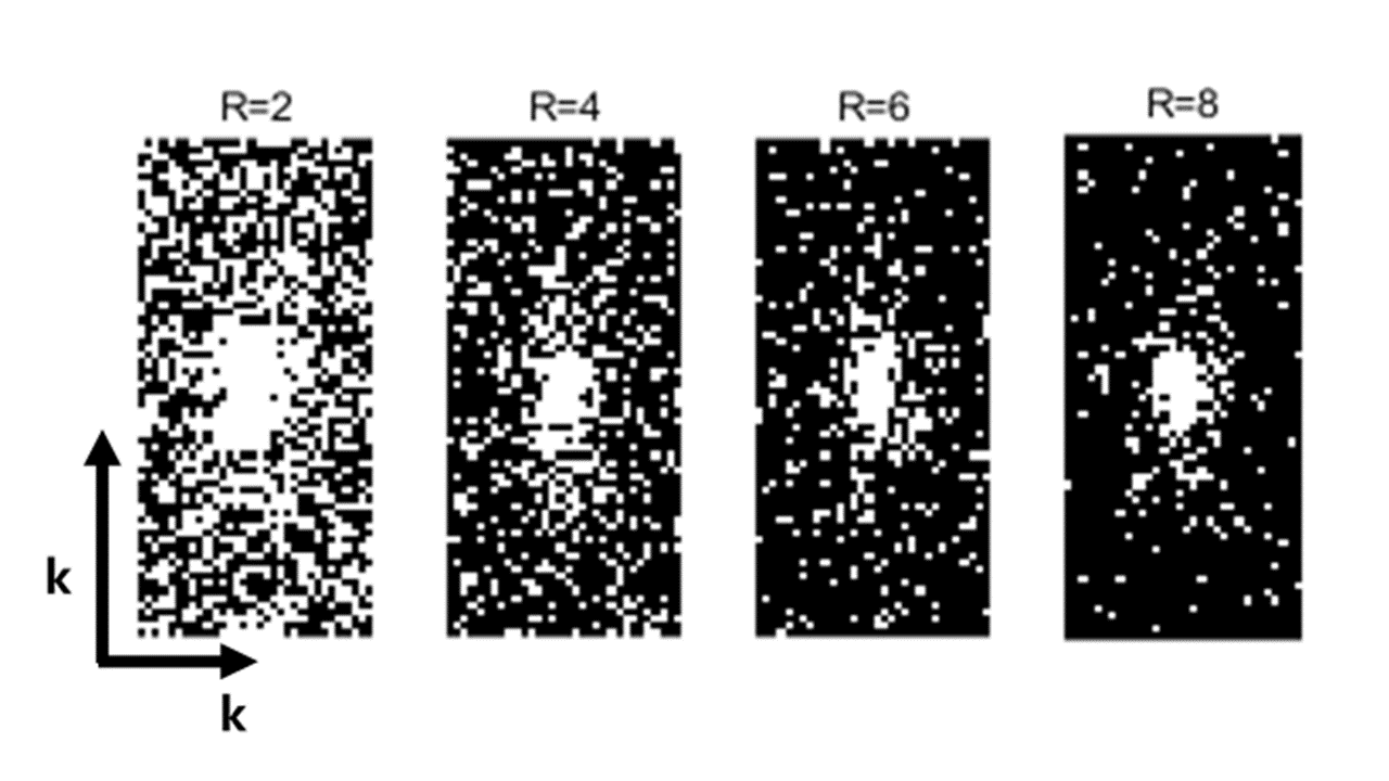
Full sampled k-space data from 4D Flow and ICOSA6 were under-sampled using 2D variable density patterns with various acceleration factors (R= 2, 4, 6, 8) as shown in Fig.2. CS reconstruction using total-variation regularization was used for the study.
[Turbulent Kinetic Energy(TKE) estimation]
Turbulent Kinetic Energy was estimated from the reconstructed images. MRI signal S(kv) in 4D flow velocity can be expressed as follows [6,7]:
$$ S(k_{v})=C\int_{-\infty}^{\infty} s(v)e^{-ik_{v}v}dv$$
where kv is level of flow sensitivity(kv= π / VENC) and C is a constant scaling factor. When turbulent flow is present in 4D flow, the intravoxel velocity variance (IVVV) of turbulent flow is expressed as follows [6,7]:
$$ \sigma ISVD=sqrt\left[\frac{2}{k_v^2}ln\left(\frac{\mid S(0)\mid}{\mid S(k_{v})\mid}\right)\right] = sqrt\overline{u_{i}\prime u_{i}\prime}$$
where S(0) is MRI signal of reference encoding (no bipolar encoding) and u_i^' indicates velocity fluctuation portion. Using this equation TKE was estimated from IVVV with fluid density ρ as follows [8]:
$$ TKE = \frac{1}{2}\rho(\overline{u_{1}\prime u_{1}\prime}+\overline{u_{2}\prime u_{2}\prime}+\overline{u_{3}\prime u_{3}\prime})$$

Results

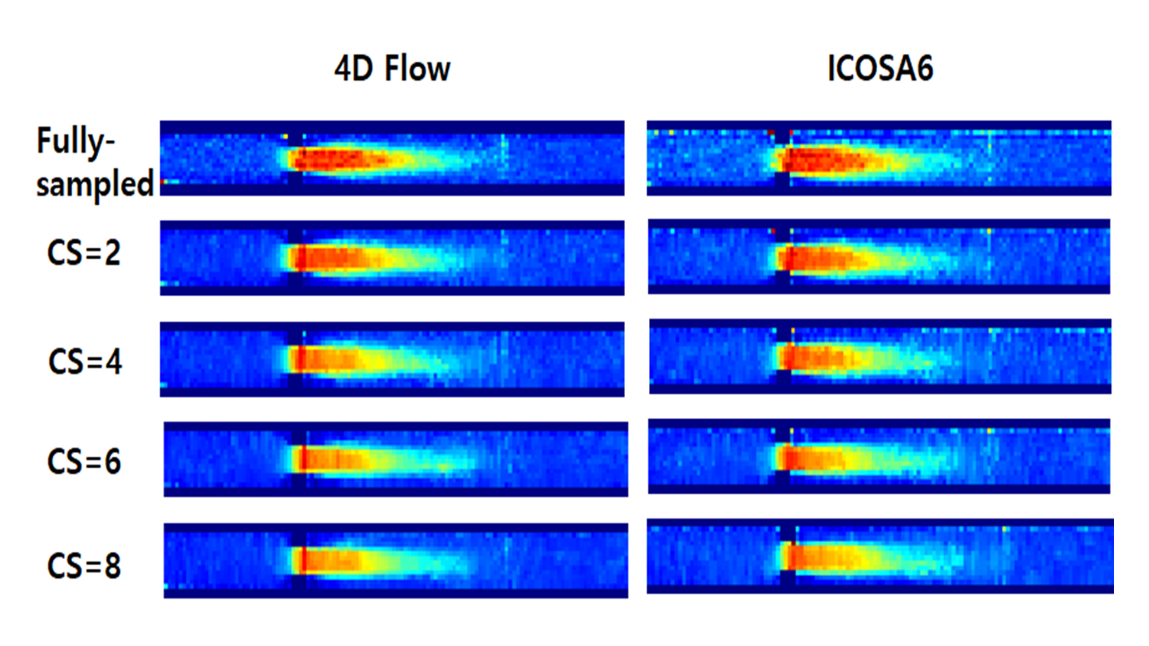
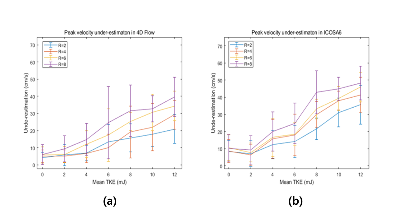
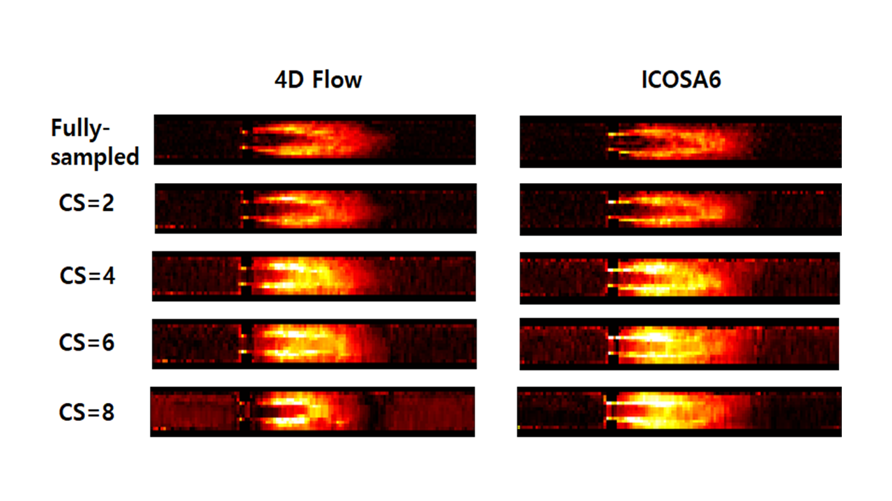
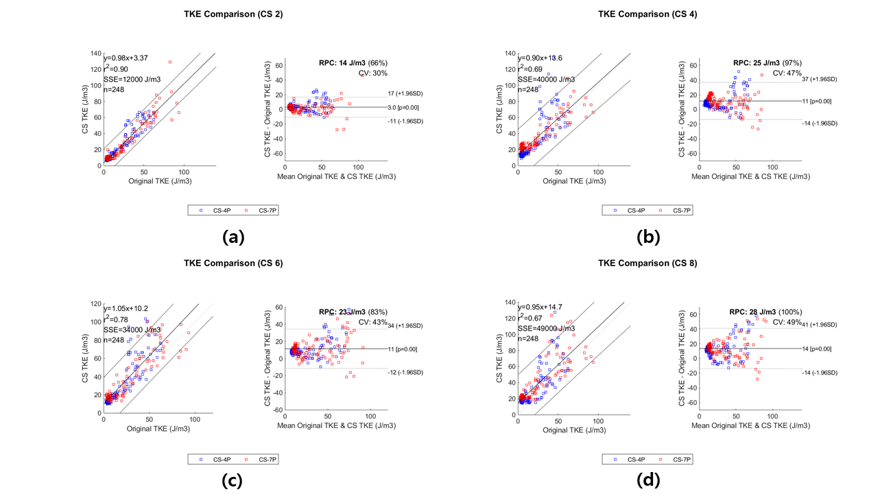
The reconstructed peak velocity images (R= 2, 4, 6, 8) and original velocity image are shown in Figure 3. Peak velocity was under-estimated along the central line. When the mean TKE increased, the gap between original velocity and CS velocity became worse as shown in Figure 4. Underestimation of peak velocity (CS= 2) increased from 4.16±3.2 (mean TKE= 0 mJ) to 20.82±8.34 (mean TKE= 12 mJ) in 4D flow, and from 8.36±6.60 (mean TKE= 0 mJ) to 35.70±11.34 (mean TKE= 12 mJ) in ICOSA6.
Images representing the TKE are shown in Figure 5 from the fully-sampled and CS reconstruction. Figure 6 shows comparison of total TKE in the central line between original and CS reconstruction in 4D Flow and ICOSA6, respectively. While the TKE images from Figure 5 show comparable results, the analysis in Figure 6 show that discrepancies between 4D versus ICOSA6 becomes aggravated beyond R=4.

Discussion and Conclusion

In this study, we explored analyzed peak velocity and turbulent flow using CS for 4D flow and ICOSA6. While ICOSA6 can give a more accurate analysis of turbulence, it is more sensitive to undersampling effects. Underestimation of peak velocity is induced due to signal loss from turbulent flow in CS reconstruction. ICOSA6 technique is more sensitive to this signal loss since it has more motion encodings. Further study for compensation method 4D flow or ICOSA6 is needed.

References

[1] Markl M, Kilner PJ, Ebbers T. Comprehensive 4D velocity mapping of the heart and great vessels by cardiovascular magnetic resonance. J Cardiovasc Magn Reson 2011;13:7.
[2] Lustig M, Donoho D, Pauly JM. Sparse MRI: the application of compressed sensing for rapid MR imaging. Magn Reson Med. 2007; 58: 1182– 1195.
[3] Tariq U, Hsiao A, Alley M, Zhang T, Lustig M, Vasanawala SS. Venous and arterial flow quantification are equally accurate and precise with parallel imaging compressed sensing 4D phase contrast MRI. J Magn Reson Imaging. 2013; 37: 1419– 1426.
[4] Ma LE, Markl M, Chow K, Huh H, Forman C, Vali A, Greiser A, Carr J, Schnell S, Barker AJ, Jin N. Aortic 4D flow MRI in 2 minutes using compressed sensing, respiratory controlled adaptive k-space reordering, and inline reconstruction. Magn Reson Med. 2019 Jun;81(6):3675-3690.
[5] E.S., Gottwald, L.M., Zhang, Q. et al. Highly accelerated 4D flow cardiovascular magnetic resonance using a pseudo-spiral Cartesian acquisition and compressed sensing reconstruction for carotid flow and wall shear stress. J Cardiovasc Magn Reson 22, 7 (2020).
[6] Dyverfeldt P, Sigfridsson A, Kvitting JPE, Ebbers T. Quantification of intravoxel velocity standard deviation and turbulence intensity by generalizing phase-contrast MRI. Magn Reson Med 2006;56(4):850–8.
[7] Binter C, Gülan U, Holzner M, SJMrim Kozerke. On the accuracy of viscous and turbulent loss quantification in stenotic aortic flow using phase-contrast MRI. 76(1). 2016. p. 191–6. [8] Pope SB. Turbulent flows. IOP Publishing; 2001.