2071
Helical Flow of Superior Vena Cava Helical Flow in Healthy Young Males: a 4D Flow MRI Study
Huaxia Pu1, Haoyao Cao2, Yubo Fan3, Jinge Zhang1, Zhenlin Li1, Zhan Liu2, Liqing Peng1, Tinghui Zheng2, Xiaoyue Zhou4, and Ning Jin5
1Department of Radiology, West China Hospital, Sichuan University, Chengdu, China, 2Department of Applied Mechanics, Sichuan University, Chengdu, China, 3Key Laboratory for Biomechanics and Mechanobiology of the Ministry of Education, School of Biological Science and Medical Engineering, Beihang University, Beijing, China, 4MR Collaboration, Siemens Healthineers Ltd, Shanghai, China, 5Siemens Medical Solutions USA, Chicago, IL, United States
1Department of Radiology, West China Hospital, Sichuan University, Chengdu, China, 2Department of Applied Mechanics, Sichuan University, Chengdu, China, 3Key Laboratory for Biomechanics and Mechanobiology of the Ministry of Education, School of Biological Science and Medical Engineering, Beihang University, Beijing, China, 4MR Collaboration, Siemens Healthineers Ltd, Shanghai, China, 5Siemens Medical Solutions USA, Chicago, IL, United States
Synopsis
The existence of helical flow in the superior vena cava (SVC) is not well understood in vivo. 4D flow MRI data of the SVC and brachiocephalic veins (BVs) were acquired in 8 healthy young males. SVC hemodynamic parameters, including velocity, pathlines, streamlines, and flow waveforms, were measured using a specialized post-processing software. Helical flow was present in the normal SVC. The flow pathlines from the right and left BVs formed helical flows, respectively, with two development types: twining and untwining. These findings may elucidate the occurrence and development of potential SVC disease.
Introduction
Helical flow has significant effect on human blood circulation, and is prominent in arterial circulation [1-4]. However, most studies of venous flow patterns rely on hydrodynamic calculations, and clinical reports related to the investigation of helical flow in the human venous system are extremely rare. As shown with central vein computational fluidics with catheter placement, flow status might be related to thrombus formation in the superior vena cava (SVC)[5, 6]. In this study, we aimed to investigate whether helical flow exists in the SVC of healthy young males, and to describe the development and characteristics of this flow pattern with 4D flow MRI.Methods
Eight healthy young males (age: 25.1 ± 4.9 years) underwent MRI on a 3T MRI (MAGNETOM Skyra, Siemens Healthcare, Erlangen, Germany). Data acquisition consisted of a prototype 4D flow sequence with retrospective ECG gating covering the SVC and brachiocephalic veins (BVs). Typical imaging parameters included: isotropic voxels (1.8 mm×2.2 mm×1.8 mm), 3D field-of-view of 276 mm×340 mm (FH x AP). TE = 2.69 - 2.79 ms, TR = 40.72 - 41.76 ms, α = 8⁰, velocity encoding = 80 cm/s, GRAPPA acceleration factor = 3, Pixel bandwidth = 490 Hz, and approximate scan time = 19 min. Hemodynamic parameters in the SVC, including velocity, velocity vectors, pathlines, streamlines, and flow waveforms, were obtained with a specialized commercial post-processing software(cvi42, version 5.11.3; Circle Cardiovascular Imaging Inc., Calgary, Canada). Data were analyzed by two experienced observers to interpret the flow pattern visually.Results
Figure 1 summarizes streamline visualization results across all subjects in the cardiac diastole, while Figure 2 shows velocity maps and streamlines chosen at 4 cardiac timepoints in two subjects. These figures demonstrate that helical flow is present in normal SVC flow, occurring in diastole. This phenomenon is mainly located at the upper and middle segments of SVC. With decreased blood velocity, helical flow area had the tendency of gradual extension. Flow pathlines originating from the left and right BVs formed helical flows, respectively, and there were two development types (Figure 3): twining (Type 1) and untwining (Type 2). Type 1 was observed in 5 cases (V2, 5-8), and involved mutual entwining of BV pathlines. Type 2 was observed in the remaining cases, and involved BV pathlines moving along the corresponding side of lumen with nearly no interference. SVC helical flow direction (Figure 4) was identified as counter-clockwise (V1-3, 5-6, left-handed) or clockwise (V4, 7-8, right-handed). SVC flow velocity was lower in the center than at the periphery. The SVC flow waveform was biphasic with some cases having centrifugal diastolic blood flow. Except for V6, the first peak of SVC flow was at cardiac time = 60.9 ± 28.5 ms (30 - 112 ms) later than peak ascending aorta flow. The emergence period of helical flow was divided into three periods corresponding to the 3 red sections in Figure 5E: initially formed helical flow, matured helical flow, and disrupted helical flow. The two BV flow waveforms were similar, but RBV flow rate was greater than that of LBV. In Type 1 helical flow, the difference between the peak flow of the two BVs was less than that of the Type 2 (8.6 ± 5.8 mL/s vs. 25.9 ± 14.5 mL/s, p=0.08).Discussion
In this study, the helical flow of SVC mainly started at the confluence of two BVs, which always appeared in pairs before gradually converging. It is considered that this natural phenomenon is caused by the mutual influence of both BVs. Aside from the peak flow difference of the two BVs, no obvious differences were observed between Type 1 and Type 2 flow patterns. Helical flow has high transport efficiency, which may help to improve the venous return rate and avoid the reduction of cardiac output [7]. Helical flow has also been recognized to inhibit blood flow disorders and instability [8, 9], which can prevent the development of chronic venous diseases by inhibiting inflammation and thrombosis. In other words, the loss of helical flow may mean an increased risk of diseases such as SVC obstruction.Conclusion
SVC visualized helical flow in healthy young males through 4D flow MRI might be a characteristic of normal physiological function in this vessel. This phenomenon has the potential to be a reference for predicting early SVC disease.Acknowledgements
This work was supported by the National Natural Science Foundation of China [grant number 81601462], 1·3·5 project for disciplines of excellence, West China Hospital, Sichuan University [ZYGD18013] and Sichuan Province Science and Technology Support plan [grant number 2016FZ0107].References
[1] A. Frydrychowicz, J.T. Winterer, M. Zaitsev, B. Jung, J. Hennig, M. Langer, M. Markl, Visualization of iliac and proximal femoral artery hemodynamics using time-resolved 3D phase contrast MRI at 3T, J Magn Reson Imaging 25(5) (2007) 1085-92. [2] P.A. Stonebridge, P.R. Hoskins, P.L. Allan, J.F. Belch, Spiral laminar flow in vivo, Clin Sci (Lond) 91(1) (1996) 17-21. [3] M. Markl, M.T. Draney, M.D. Hope, J.M. Levin, F.P. Chan, M.T. Alley, N.J. Pelc, R.J. Herfkens, Time-resolved 3-dimensional velocity mapping in the thoracic aorta: visualization of 3-directional blood flow patterns in healthy volunteers and patients, J Comput Assist Tomogr 28(4) (2004) 459-68. [4] M.S. Wetzel S, Frydrychowicz A, Bonati L, Radue EW, Scheffler K, Hennig J, Markl M, In vivo assessment and visualization of intracranial arterial hemodynamics with flow-sensitized 4D MR imaging at 3T., American Journal of Neuroradiology 28(3) (2007) 433-438. [5] L. Peng, Y. Qiu, Z. Huang, C. Xia, C. Dai, T. Zheng, Z. Li, Numerical Simulation of Hemodynamic Changes in Central Veins after Tunneled Cuffed Central Venous Catheter Placement in Patients under Hemodialysis, Sci Rep 7(1) (2017) 15955. [6] M. Park, Y. Qiu, H. Cao, Y. Ding, D. Li, Y. Jiang, L. Peng, T. Zheng, Influence of Hemodialysis Catheter Insertion on the Hemodynamics in the Central Veins, J Biomech Eng (2020). [7] X. Liu, A. Sun, Y. Fan, X. Deng, Physiological significance of helical flow in the arterial system and its potential clinical applications, Ann Biomed Eng 43(1) (2015) 3-15. [8] M. Brass, Z.C. Berwick, X. Zhao, H. Chen, J. Krieger, S. Chambers, G.S. Kassab, Growth and remodeling of canine common iliac vein in response to venous reflux and hypertension, J Vasc Surg Venous Lymphat Disord 3(3) (2015) 303-311 e1. [9] G. De Nisco, A. Hoogendoorn, C. Chiastra, D. Gallo, A.M. Kok, U. Morbiducci, J.J. Wentzel, The impact of helical flow on coronary atherosclerotic plaque development, Atherosclerosis 300 (2020) 39-46.Figures
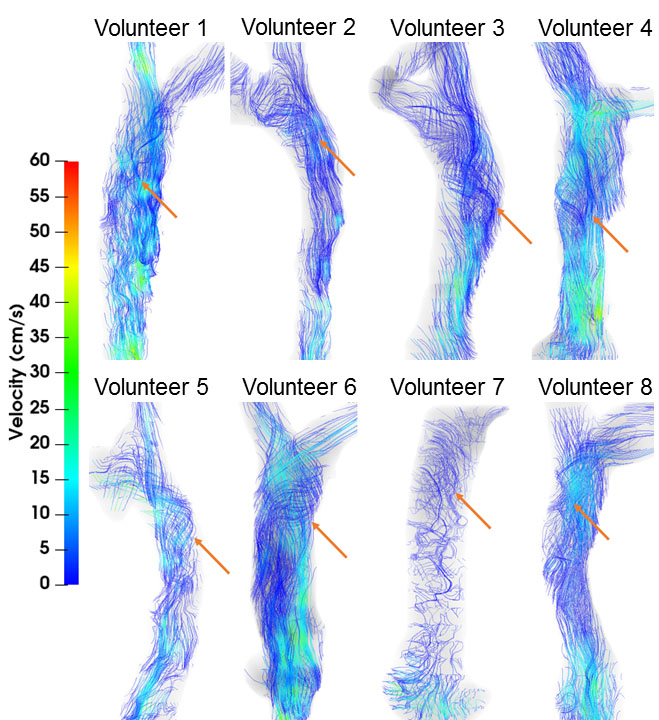
Figure 1. Streamline visualizations (color-coded to blood speed) in all 8
subjects. Helical flow (red arrows) was observed in all subjects.
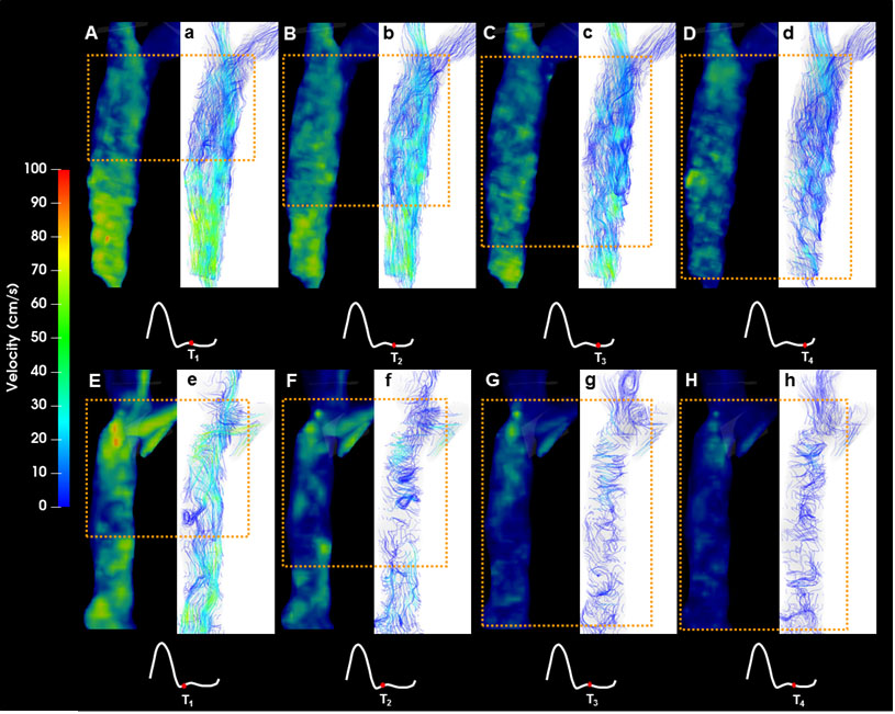
Figure 2. Example color-coded velocity maps in the superior
vena cava in two volunteers (V1: A-D, V5: E-H) and corresponding streamline visualization
images (V1: a-d, V5: e-h) at four cardiac timepoints throughout the cardiac
cycle. Yellow rectangles indicate helical flow location. Acquisition times of
the corresponding images (as % of R-R interval) were: upper row (V1) T1
= 64.5%, T2 = 70.8%, T3 = 77.0%, T4 = 83.2;
lower row (V5): T1 = 48.2%; T2 = 54.2%; T3 =
59.9%; T4 = 66.2%.
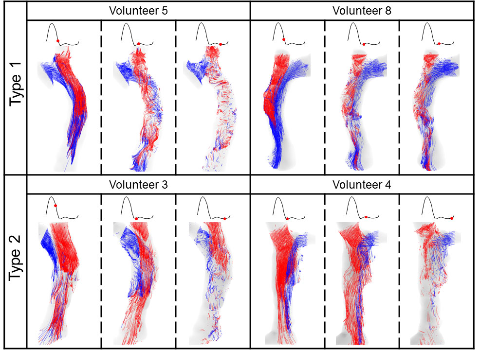
Figure 3. Superior vena cava pathline visualizations in 4
volunteers at three cardiac timepoints each, showing (from
left to right) no helical flow, matured helical flow, and disrupted helical
flow, respectively. Type 1 (twining) is shown in the top row, and Type 2
(untwining) in the bottom row.
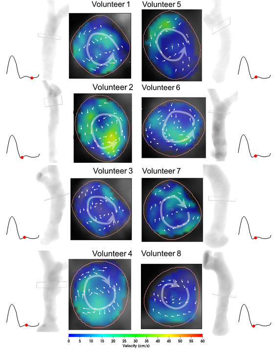
Figure 4. Example superior vena cava cross-sectional fusion
images of velocity vector visualization and velocity maps (middle
two columns), with the direction of helical flows (white curved arrow) shown.
Location for each cross-section is shown (white transparent rectangle) on the
vessel maximum intensity projection. Images are exhibited at individual
timepoints (red dots) in the cardiac cycle.
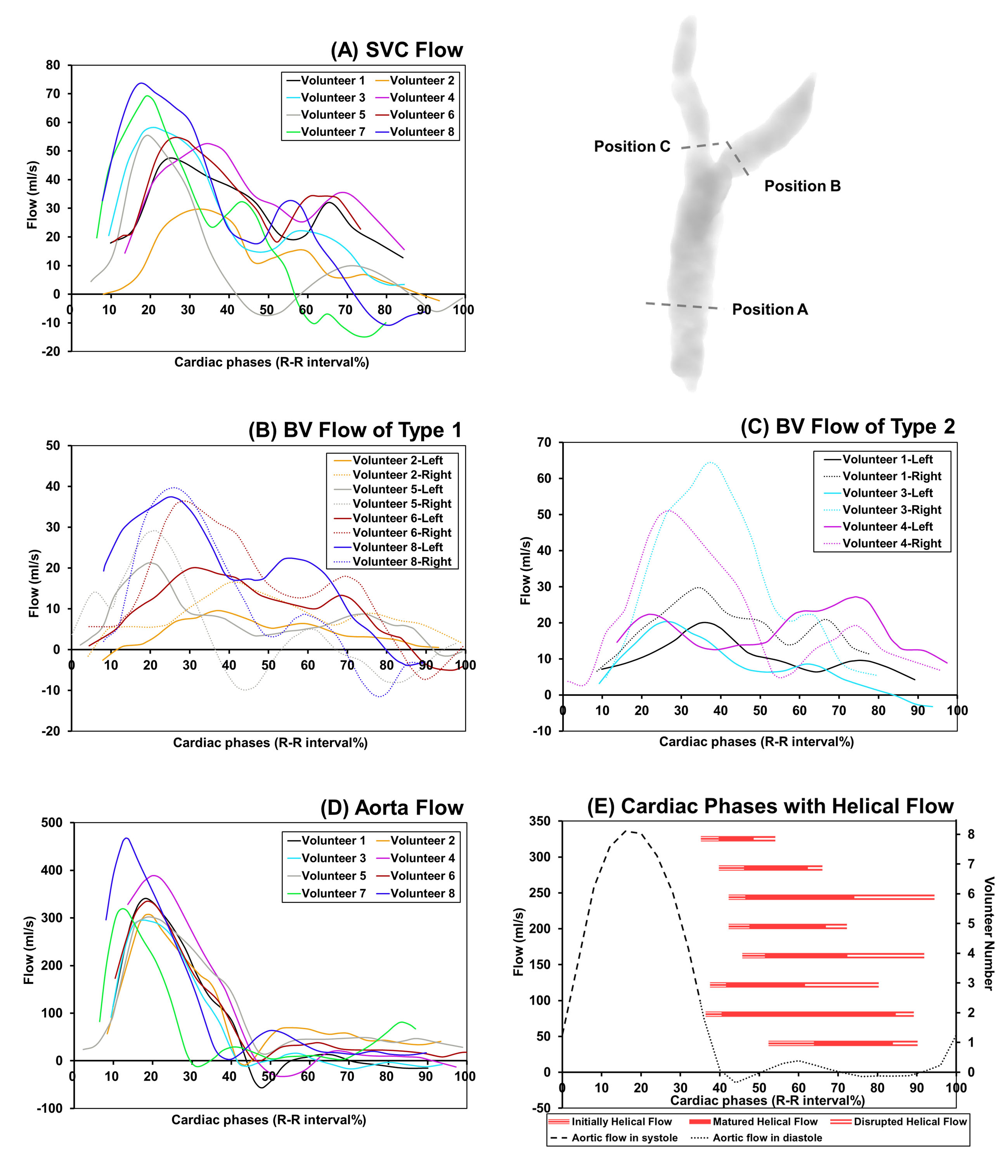
Figure 5. (A)
Flow waveforms of SVC measured at Position A. (B) Flow waveforms of two BVs in
Type 1, and (C) flow waveforms of two BVs in Type 2. LBVs (solid line) were
measured at Position B, while RBVs (dotted lines) were measured at Position C. (D)
Ascending aorta flow waveforms, and (E) corresponding to the
cardiac phases with helical flow. Note: As the LBV and RBV were not covered
during the scan, the flow waveforms of two BVs of Volunteer 7 are not
displayed.