2041

Susceptibility-induced fiber orientation dependency of the DWI signal in white matter measured in ex vivo rat brain at 7 T

Sidsel Winther^1,2, Mariam Andersson^1,2, Henrik Lundell², and Tim Dyrby^1,2
¹DTU Compute, Technical University of Denmark, Kongens Lyngby, Denmark, ²Danish Research Center for Magnetic Resonance, Functional and Diagnostic Imaging and Research, Copenhagen University Hospital Hvidovre, Hvidovre, Denmark

Synopsis

Magnetic susceptibility of myelin induces morphology- and orientation-dependent perturbations of the B_0-field. At the microstructural scale of brain white matter, the main contribution to these perturbations comes from myelin. Here, we show that a consequence of this is a fiber-orientation-dependent bias of the DWI-signal across white matter regions in an ex vivo rat brain. This implies that biophysical modeling must regard susceptibility at the microstructural scale in order not to become biased as well. Higher field strength will increase the bias and vice versa. Hence, especially pre-clinical scans are affected.

Introduction

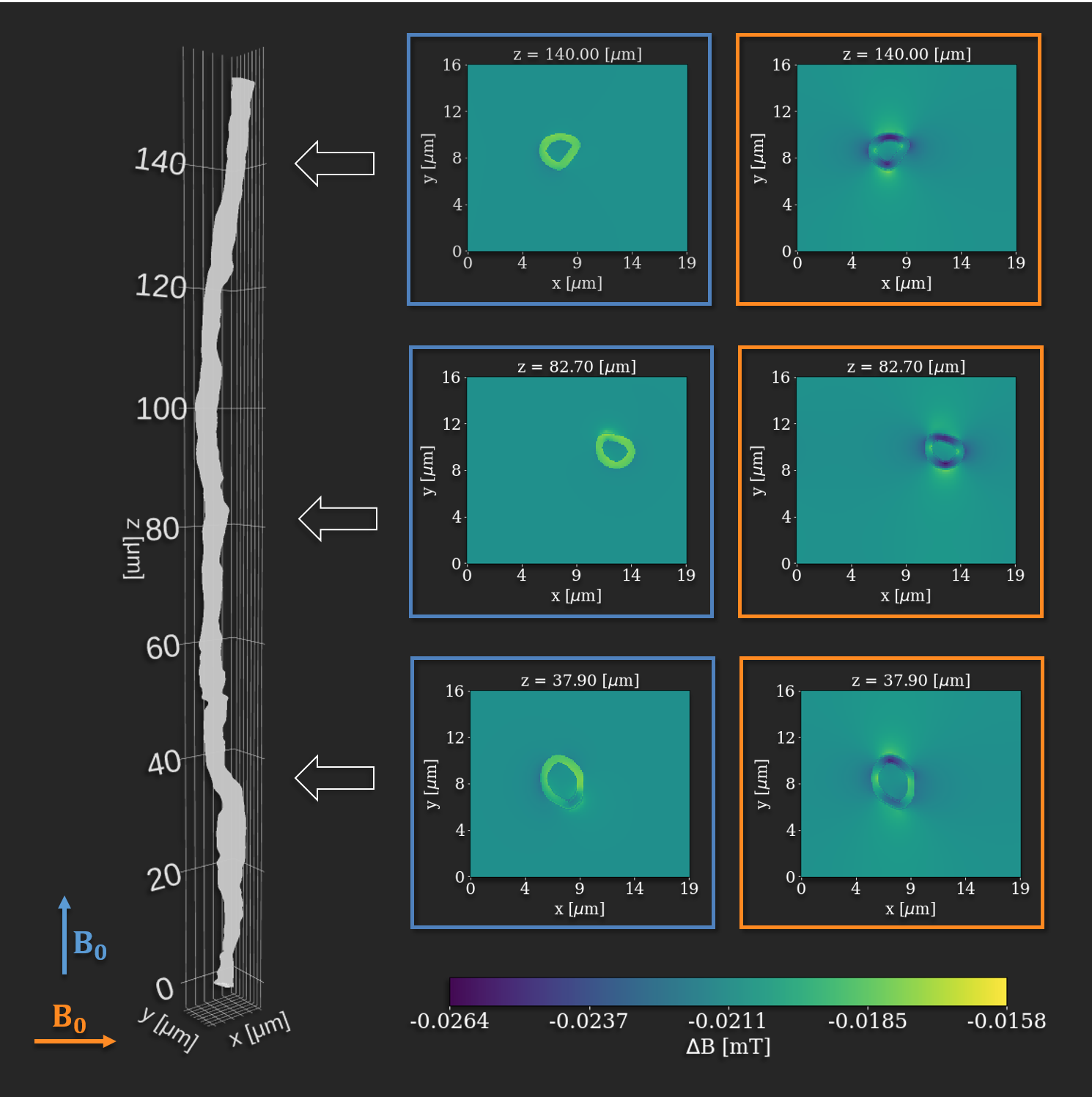
With a sufficient number of uniformly distributed b-vectors it is commonly assumed that the acquired DWI signal and the related biophysical modeling is independent of sample orientation ^1,2. However, magnetic susceptibility induces morphology- and orientation-dependent perturbations of the $$$B_0$$$-field ^3,4. At the microstructural scale of brain white matter (WM), the main contribution to these perturbations comes from myelin ⁵. Hence, WM areas of different composition (anisotropy, fiber directions, axon diameters, etc.) will be affected differently. This leads to an orientation-dependent bias. Such effects have been shown for DWI theoretically and with simulations ^6,7. We have previously shown a significant effect in simulated DWI data of straight hollow cylinders ⁸. Here, we show similar effects in an ex vivo rat brain.

Figure 1 shows how an axon from the corpus callosum (CC) of a vervet monkey (segmented from 3D x-ray nano-holotomography) ⁹ perturbs the applied $$$B_0$$$-field when oriented parallel or perpendicular to the field ⁸. From these results we know that the field, and hence the signal, will be most affected when fibers are oriented perpendicular to the applied field, and least affected when oriented parallel to the applied field. The results also demonstrate that the gradients in the perturbed field are stronger perpendicular to the axon than parallel to it. It is known that higher field strength will increase the perturbations and vice versa. Areas with higher anisotropy (lower global and/or local fiber dispersion) are affected most.

Methods

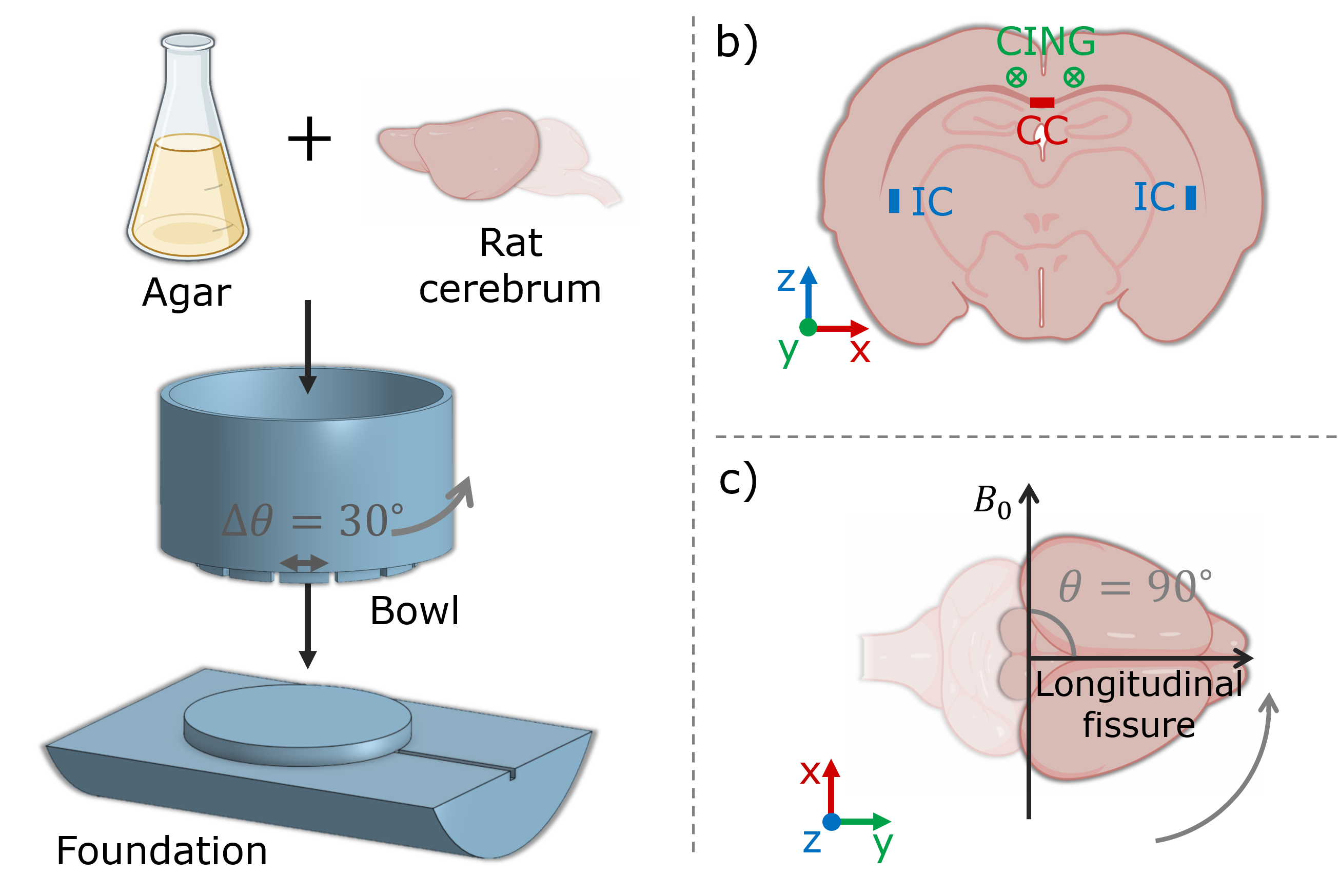
Sample: A post mortem rat brain was scanned. Perfusion fixation and storage was performed as in ¹⁰. The brain was rinsed with KPBS before scanning. Cerebellum and brain stem were removed. The brain was installed in a rotation device by molding it in a 2% agar solution; ensuring stable rotation, and centering within the coil. See Figure 2, a.

MRI: Scans were performed with a Bruker Biospec 70/20 7T scanner, and a quadrature coil. Images were acquired with a 2D sequence of 200 μm isotropic resolution (slices along z). The following parameters were applied for a PGSE-sequence: $$$\delta$$$=5.3 ms, $$$\Delta$$$=12.0 ms, TE=31.8 ms, TR=2600.0 ms, BW=18518.5 Hz, and prescribed b-values were (300, 2000, 3000, 4000) s/mm$$$^2$$$. Diffusion encoding directions were given as 21 uniformly distributed b-vectors projected in positive z-direction and repeated for opposite polarities in order to correct for cross-terms with linear background and imaging gradients ¹¹. Scans were repeated with different orientations with respect to $$$B_0$$$: (0, 90, 30, 60) degrees (Figure 2, c). Acquired in random order to minimize temporal bias in the analysis. For each scan the field of view (FOV) was aligned with the orientation of the brain.

Analysis: We focus on fibers in the orthogonal directions x, y, and z, corresponding to midsagittal corpus callosum (CC), cingulum bundle (CING), and internal capsule (IC) respectively (Figure 2, b). Voxels of interest are extracted based on manual selection, and thresholding criteria: normalized signal >0.22 at lowest b-value, FA >0.60, and angle with respect to the fiber-direction of interest <20 degrees.

Results and discussion

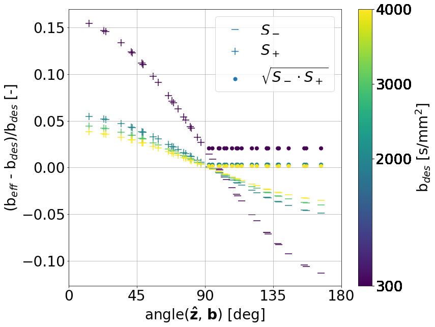
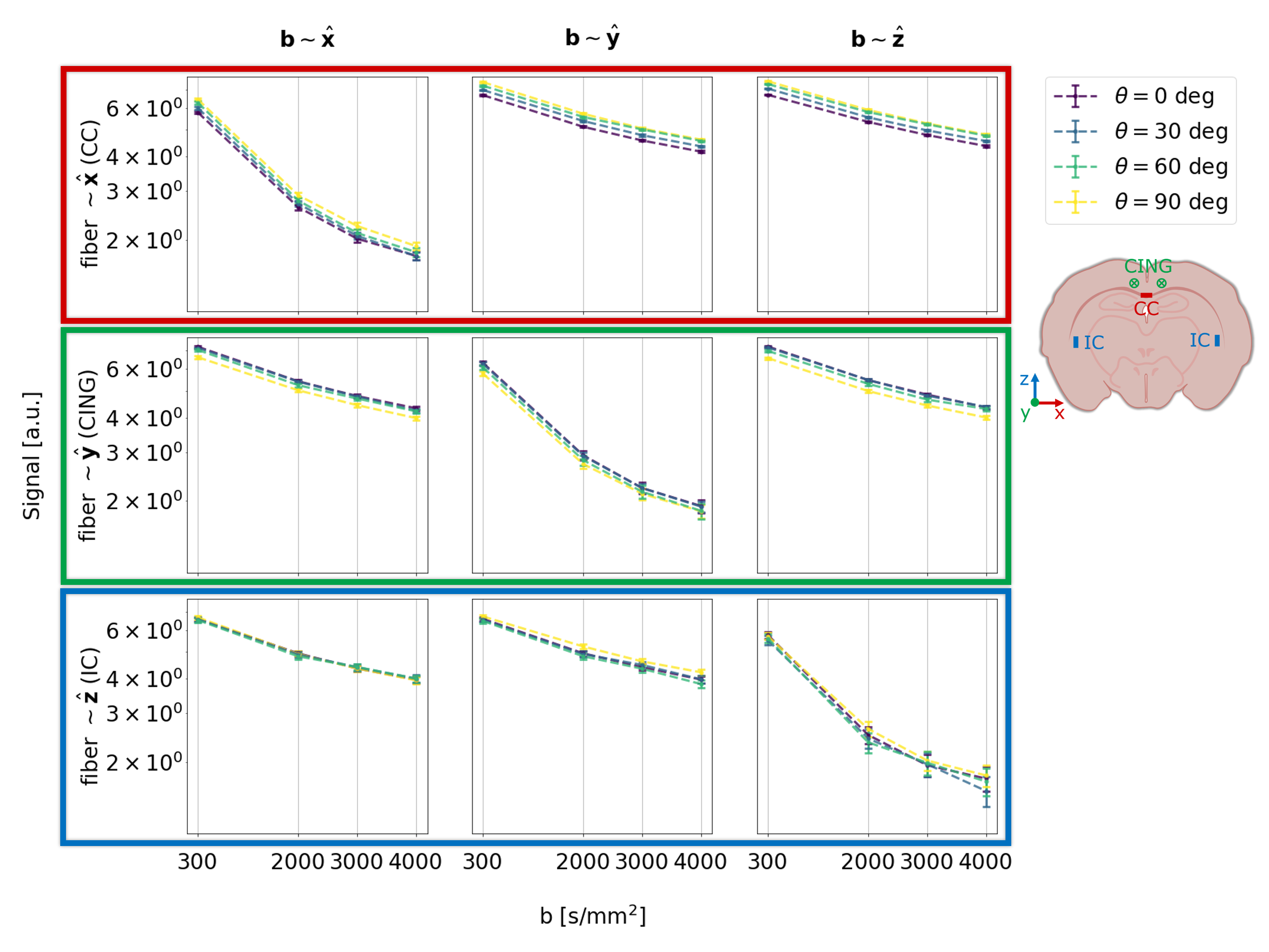
With increasing resolution of 2D imaging the effective b-values become substantially skewed along the slice-direction due to the superposition of diffusion gradients and image slicing gradients. These effects are partially corrected by the opposite polarity correction (Figure 3).

Figure 4 shows the raw signal. 1st, 2nd, and 3rd row show the signal from CC, CING, and IC, respectively. 1st, 2nd, and 3rd column show the signal from the b-vectors closest to x, y, and z, respectively. Hence, the diagonal shows the signal measured parallel to the fibers, and the off-diagonal shows signal measured perpendicular to the fibers.

For CC we see that the signal is highest when $$$\theta$$$=90 deg (and the fibers of CC are parallel to $$$B_0$$$), and decreases as $$$\theta$$$ decreases to 0 deg (and the fibers of CC are perpendicular to $$$B_0$$$). As we expect from the results shown in Figure 1, where the susceptibility-induced gradients are largest when the fiber is perpendicular to $$$B_0$$$. The signal measured with b-vectors perpendicular to the fibers is affected more than the signal measured parallel to the fibers. As we expect from the results shown in Figure 1, where the gradients are strongest perpendicular to the axon.

For CING the effect is opposite of CC; as expected, since the two are oriented perpendicular to each other in the plane of rotation w.r.t. $$$B_0$$$.

For IC, no systematic orientation dependency is observed; as expected, because the rotations w.r.t. $$$B_0$$$ causes minimal variations around z.

The primary effect of the varying orientation is expressed as a T2* effect. The orientation-dependency is in qualitative correspondence with the findings for R2* by Rudko et al. ¹².

Conclusions

An orientation-dependent bias of PGSE-acquired DWI-signal was observed for anisotropic white matter structures of an ex vivo rat brain. The bias is in correspondence with the qualitative expectations for susceptibility-induced $$$B_0$$$-field perturbations of the analyzed regions. A consequence of this is a fiber-orientation-dependent bias of the DWI-signal across the brain. This implies that global biophysical modeling is infeasible without correcting for this bias.

Acknowledgements

MA and TD have received funding from the Capital Region Research Foundation (grant number A5657). HL has received funding from the European Research Council (ERC) under the European Union’s Horizon 2020 research and innovation programme (grant agreement No 804746).

References

1. P. Basser, et al. MR diffusion tensor spectroscopy and imaging. Biophysical Journal, 1994;66(1):259–267.

2. F. Szczepankiewicz, et al. Minimum number of diffusion encoding directions required to yield a rotationally invariant powder average signal in single and double diffusion encoding. ISMRM, 2016.

3. S. Blundell. Magnetism in condensed matter. Oxford master series in condensed matter physics. Oxford University Press, Oxford, repr. edition, 2001.

4. J. Schenck. The role of magnetic susceptibility in magnetic resonance imaging: MRI magnetic compatibility of the first and second kinds. Medical Physics, 1996;23(6):815–850.

5. T. Xu, et al. The effect of realistic geometries on the susceptibility-weighted MR signal in white matter. Magnetic Resonance in Medicine, 2018;79(1):489–500.

6. J. Trudeau, et al. The Effect of Inhomogeneous Sample Susceptibility on Measured Diffusion Anisotropy Using NMR Imaging. Journal of Magnetic Resonance, Series B, 1995;108(1):22-30.

7. D. Novikov, et al. Effects of mesoscopic susceptibility and transverse relaxation on diffusion NMR. Journal of Magnetic Resonance, 2018;293:134–144.

8. S. Winther, et al. Orientation-dependent biases in powder averaging caused by inhomogeneous distributions of magnetic susceptibility in white matter. ISMRM, 2020.

9. Andersson, M. et al. Axon morphology is modulated by the local environment and impacts the non-invasive investigation of its structure-function relationship. Proc. Natl. Acad. Sci. U. S. A. In Press.

10. T. Dyrby, et al. An ex vivo imaging pipeline for producing high-quality and high-resolution diffusion-weighted imaging datasets. Human Brain Mapping, 2011;32(4):544-63.

11. H. Jara, et al. Determination of background gradients with diffusion MR imaging.JMRI, 1994;4(6):787-797.

12. D. Rudko, et al. Origins of R2* orientation dependence in gray and white matter. Proc. Natl. Acad. Sci. U. S. A, 2014;111(1):159-167.

Figures

Figure 1: Left: Axon from the corpus callosum of a vervet monkey brain (segmented from 3D x-ray nano-holotomography). Right: Cross-sections of the perturbations $$$\Delta B$$$ of an applied field of 7 T computed with 0.1 μm isotropic resolution with an in-house software for parallel (blue) and perpendicular (orange) orientation w.r.t. the field. The field is most affected when fibers are oriented perpendicular to the field. The gradients are stronger perpendicular to the axon than parallel to it.

Figure 2: Experimental setup. a) Rotation device tailored for the MR-coil such that the center of the bowl is the center of the coil. Cerebrum was molded in agar to stabilize it in the bowl. The bowl was placed on a foundation to control the rotation. b) Axial cross-section of a schematic rat brain. ROIs are marked and color-coded. c) The orientation of the brain w.r.t. The $$$B_0$$$ field is measured as the angle $$$\theta$$$ between $$$B_0$$$ and the longitudinal fissure.

Figure 3: Each mark represents the b-value of an individual b-vector. y-axis: The relative deviation between the effective b-values ($$$b_{eff}$$$) and the desired b-values ($$$b_{des}$$$). x-axis: The angle between $$$\hat{\mathbf{z}}$$$ and the b-vector. $$$S_-$$$ refers to the b-vectors located on the negative hemisphere of a z-oriented sphere. $$$S_+$$$ refers to those located on the positive hemisphere. Dots refer to the b-values obtained from opposite polarity correction.

Figure 4: 1st, 2nd, and 3rd row shows the signal from CC, CING, and IC, respectively. 1st, 2nd, and 3rd column show the signal from the b-vectors closest to x, y, and z, respectively. Hence, the diagonal shows the signal measured parallel to the fibers, and the off-diagonal shows signal measured perpendicular to the fibers. Each point represents the average of all voxels of interest. Number of voxels varied across scans: 681 to 816, 209 to 283, and 64 to 93 for CC, CING, and IC, respectively.

Proc. Intl. Soc. Mag. Reson. Med. 29 (2021)

2041