2021
On the quantification of the striatum neurochemical profile using STEAM MRS: a comparison of 3T versus 7T in a cohort of elderly subjects1Institute of Neuroscience and Medicine 4, Medical Imaging Physics, Forschungszentrum Jülich, Jülich, Germany, 2Engineering Physics Department, Georgian Technical University, Tbilisi, Georgia, 3Institute of Neuroscience and Medicine 3, Forschungszentrum Jülich, Jülich, Germany, 4University of Cologne, Faculty of Medicine and University Hospital Cologne, Department of Neurology, Cologne, Germany, 5Institute of Neuroscience and Medicine 11, Forschungszentrum Jülich, Jülich, Germany, 6JARA BRAIN Translational Medicine, RWTH Aachen University, Aachen, Germany, 7Department of Neurology, Faculty of Medicine, RWTH Aachen University, Aachen, Germany
Synopsis
The primary aim of this study is to quantify the neurochemical profile of the human striatum in vivo in healthy subjects, using data acquired with a single voxel STEAM MRS sequence at 3T and 7T in a case-control study on Parkinson’s disease. Given that the voxel sizes at both fields were different, we intend to ascertain the conditions under which the neurochemical profiles at 3T and 7T are comparable. To this end, we assessed different quantification methods and strategies, including correction for transverse and longitudinal relaxation and for differences in grey and white matter metabolite concentrations.
Introduction
The use of the unsuppressed tissue water signal as an internal reference in 1H magnetic resonance spectroscopy (MRS)1 has been shown to be of great value for quantifying the metabolic profile in vivo. However, a limitation of this approach is the assumption that the metabolite concentration in all tissues covered by the voxel is the same.2 In order to overcome this limitation, Harris et al.3 proposed adding a factor equal to the ratio of the metabolite concentration in white (WM) and grey matter (GM).The aim of this work was to quantify the neurochemical profile of the human striatum in vivo, using data from the healthy control subjects of a Parkinson’s disease study, acquired using the single voxel stimulated echo acquisition mode (STEAM)4,5 sequence at 3T and 7T. Given that the voxel sizes and sequence timings at both field strengths were different, we investigate the conditions under which the measured concentrations at both field strengths can be compared. First we assess the differences in concentration between GM and WM following Ref.2 and use the method proposed by Harris et al.3 for quantification.
Materials and Methods
We compared three quantification methods. The first one (M1) accounts for differences in water concentration in different tissues.6 The absolute concentration of a given metabolite, m, is given by:$$c_{\mathrm{m},1}={\rm LCM}_\mathrm{OUT}\ \frac{\sum_{i}{c_{w,i}f_i}}{f_\mathrm{GM}\ +\ f_\mathrm{WM}}$$
where LCMOUT is the LCModel concentration output, $$$i$$$=WM, GM and CSF, $$$c_{w,i\ }$$$ is the water concentration in WM/GM/CSF = 36100/43300/53800mM, and $$$f_i$$$ is the tissue volume fraction.
The second method (M2) incorporates a correction for relaxation effects:3
$$c_{\mathrm{m},2}={\rm LCM}_\mathrm{OUT}\frac{\sum_{i}{c_{w,i}R_{1,i}R_{2,i}f_i}}{R_\mathrm{1,m}R_\mathrm{2,m}\ (f_\mathrm{GM}+f_\mathrm{WM})}$$
where R1 and R2 for STEAM are written as:
$$R_1=\left(1-\exp\left[\left(\frac{\mathrm{TE}}{2}+\mathrm{TM}-\mathrm{TR}\right)\frac{1}{T_1}\right]\right)\exp\left(-\frac{\mathrm{TM}}{\mathrm{T_1}}\right); \quad R_2=\mathrm{exp\left(-\frac{TE}{T_2}\right)}$$
and T1 and T2 are the relaxation times and TE, TM and TR are the echo, mixing and repetition times.
The third method (M3) additionally considers that metabolite concentration in WM and GM are different3
$$c_\mathrm{m,3}={\rm LCM}_\mathrm{OUT}\frac{\sum_{i}{c_{w,i}R_{1,i}R_{2,i}f_i}}{R_\mathrm{1,m}R_\mathrm{2,m}\ (f_\mathrm{GM}+\alpha_\mathrm{m}f_\mathrm{WM})}$$
where $$$\alpha_\mathrm{m}={c_\mathrm{{m,WM}}}\diagup{c_{\mathrm{m,GM}}}$$$ is the concentration ratio.
MRS spectra were acquired from the striatum of 14 healthy subjects in the framework of a Parkinson’s disease study after obtaining written, informed consent. Given that the covered range of tissue fractions for this study was small, we included five additional subjects, for which the voxel was deliberately shifted to include higher fractions of WM.
Experiments were performed in a Siemens 3T hybrid PET/MR scanner (Siemens, Erlangen, Germany) and in a 7T Siemens Terra scanner. An MPRAGE7 sequence was used to position the voxel at 3T (TE/TR=2.89ms/2.5s; voxel-size=13mm3), and an MP2RAGE8 sequence was used at 7T (TE/TR=1.99ms/4.5s; voxel-size=0.753mm3).
B0 shimming was performed using FASTESTMAP.9 The radiofrequency power was calibrated for each subject.10 Spectra were measured using STEAM. Protocol parameters for 3T were: TE/TR/TM=6/4800/47.82ms; 128 averages; voxel-size=21×35×21mm3; receive-bandwidth, 6000 Hz; vector-size=2048. For 7T were: TE/TR/TM=4/8000/28ms, 72 averages; voxel-size=14×32×17mm3; receive-bandwidth, 6000 Hz; vector-size=2048. One extra measurement without the water suppression was performed for eddy-current correction and absolute quantification.
All data were pre-processed in Matlab with the help of the FID-A11 package. Quantification was performed using LCModel. All basis sets were generated with the help of VeSPA12 using the density matrix formalism13 with ideal pulses and actual sequence timings.14-16 Macromolecules spectra measured using STEAM and comparable experimental parameters17 (https://github.com/mrshub/mm-consensus-data-collection ) were used. A metabolite was considered to be reliably estimated if it was detected in 50% of the subjects with a CRLB value <50%. Spectra with water linewidth >0.07ppm were discarded. For evaluating the tissue volume fractions, we combined two segmentation approaches, namely FAST18 for cortical GM and FIRST19 for subcortical structures.20 A two-sample t-test was used to assess field differences.
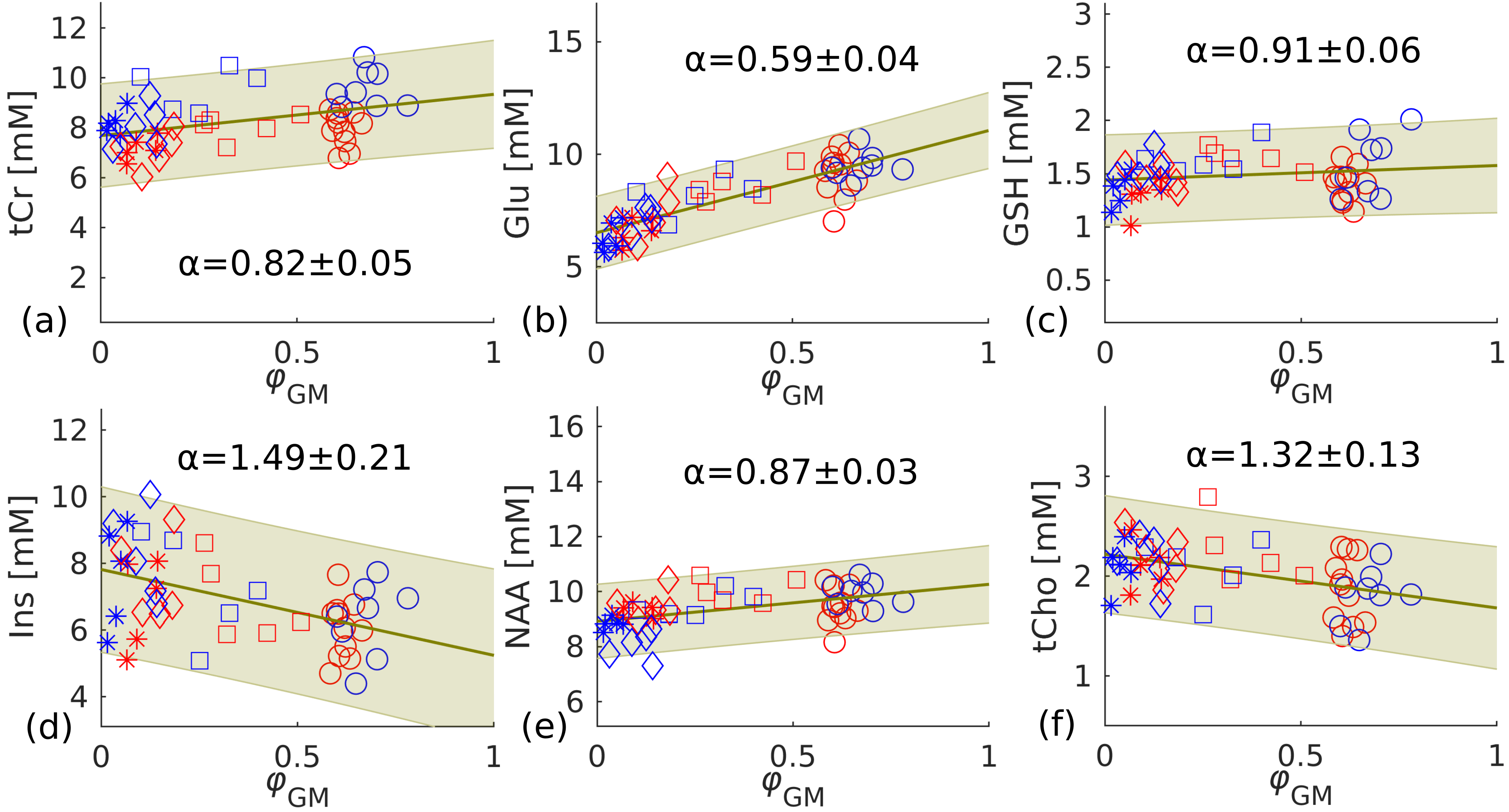
For the estimation of αm, metabolites were first quantified with M2 using literature relaxation parameters.21-24 Then concentrations were plotted against the normalised volume fraction, $$$\varphi_\mathrm{GM}={f_\mathrm{GM}}\diagup{\left(f_\mathrm{GM}+f_\mathrm{WM}\right)}$$$, and a linear regression was performed.1,2 The concentration of each metabolite for pure GM and WM could then be obtained from the fitting results.
Results
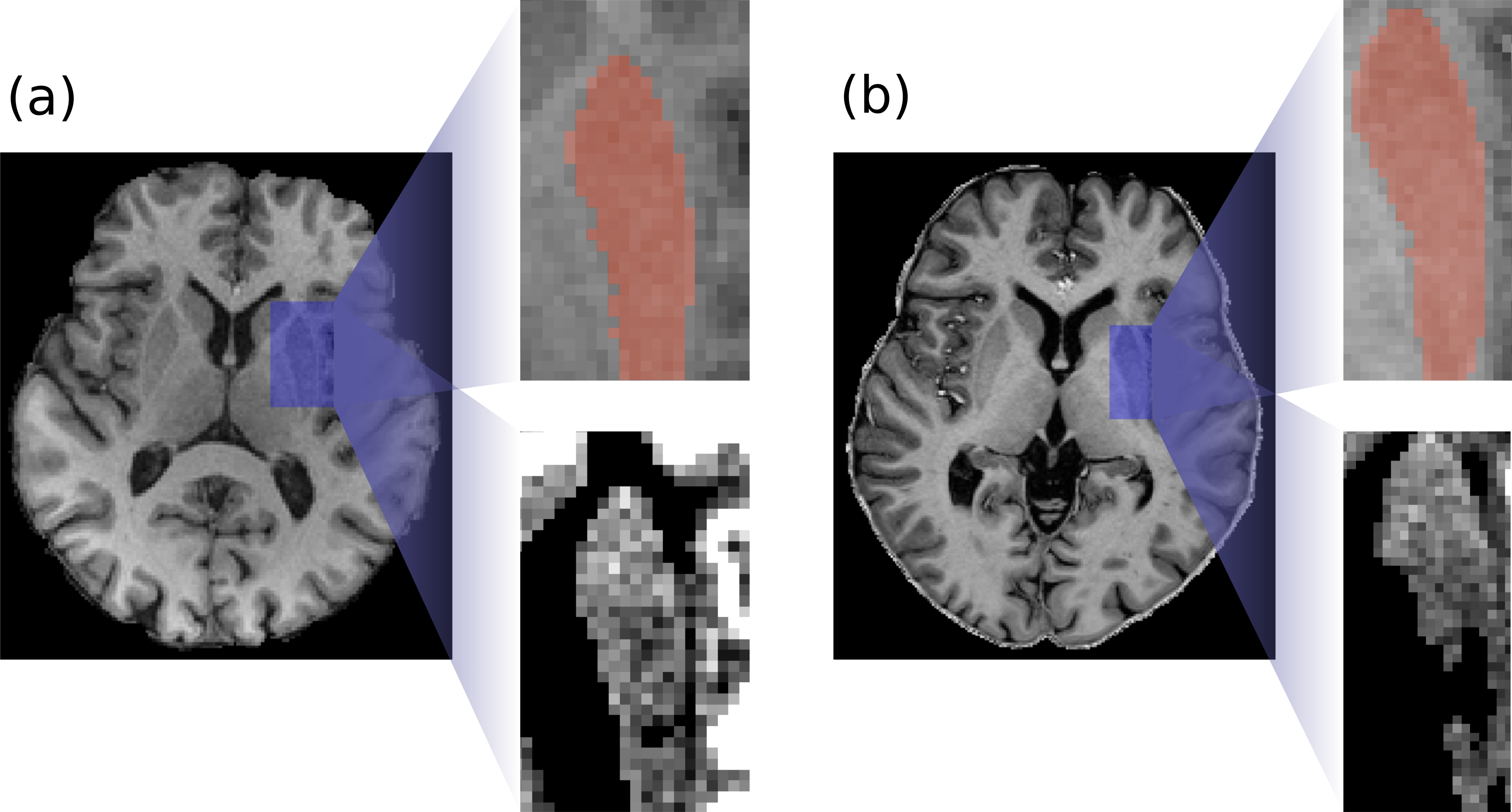
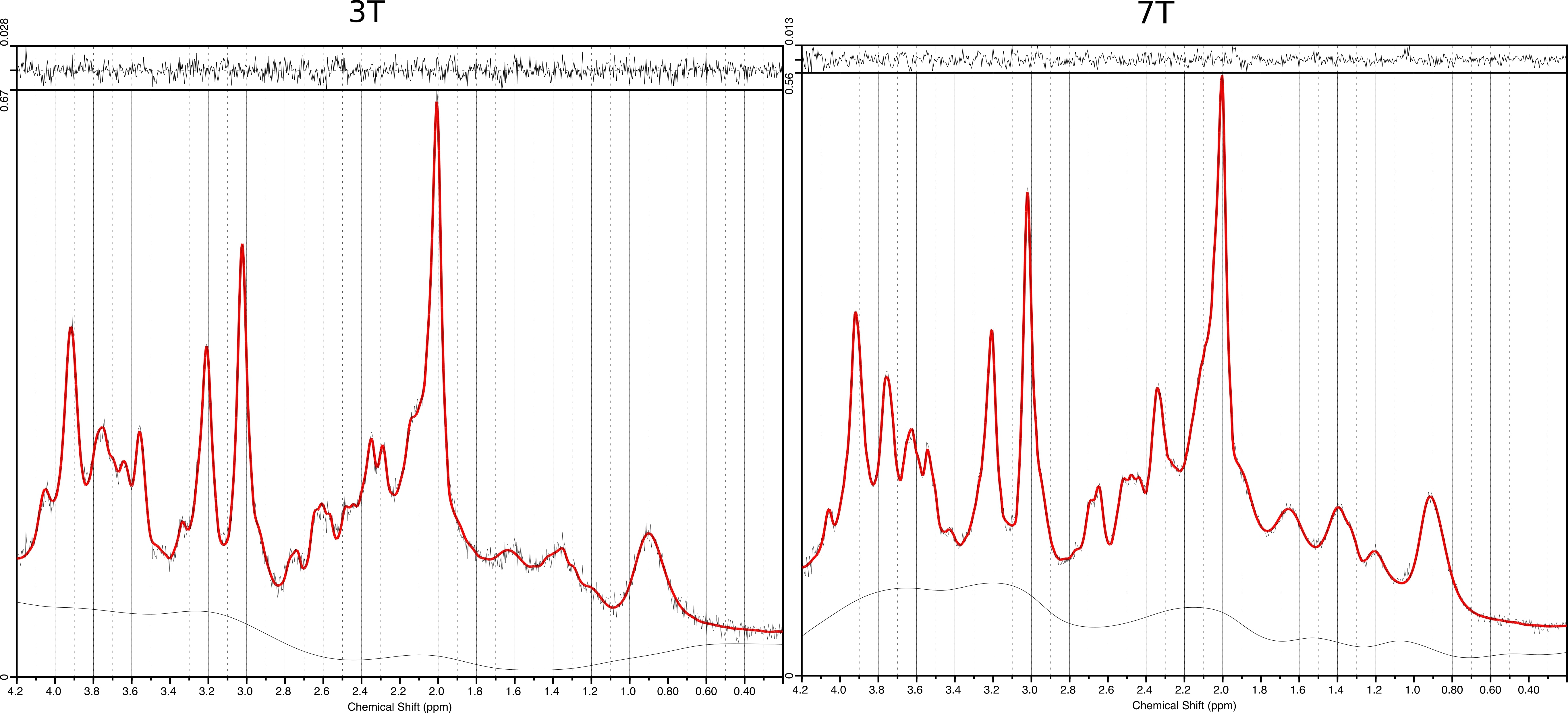
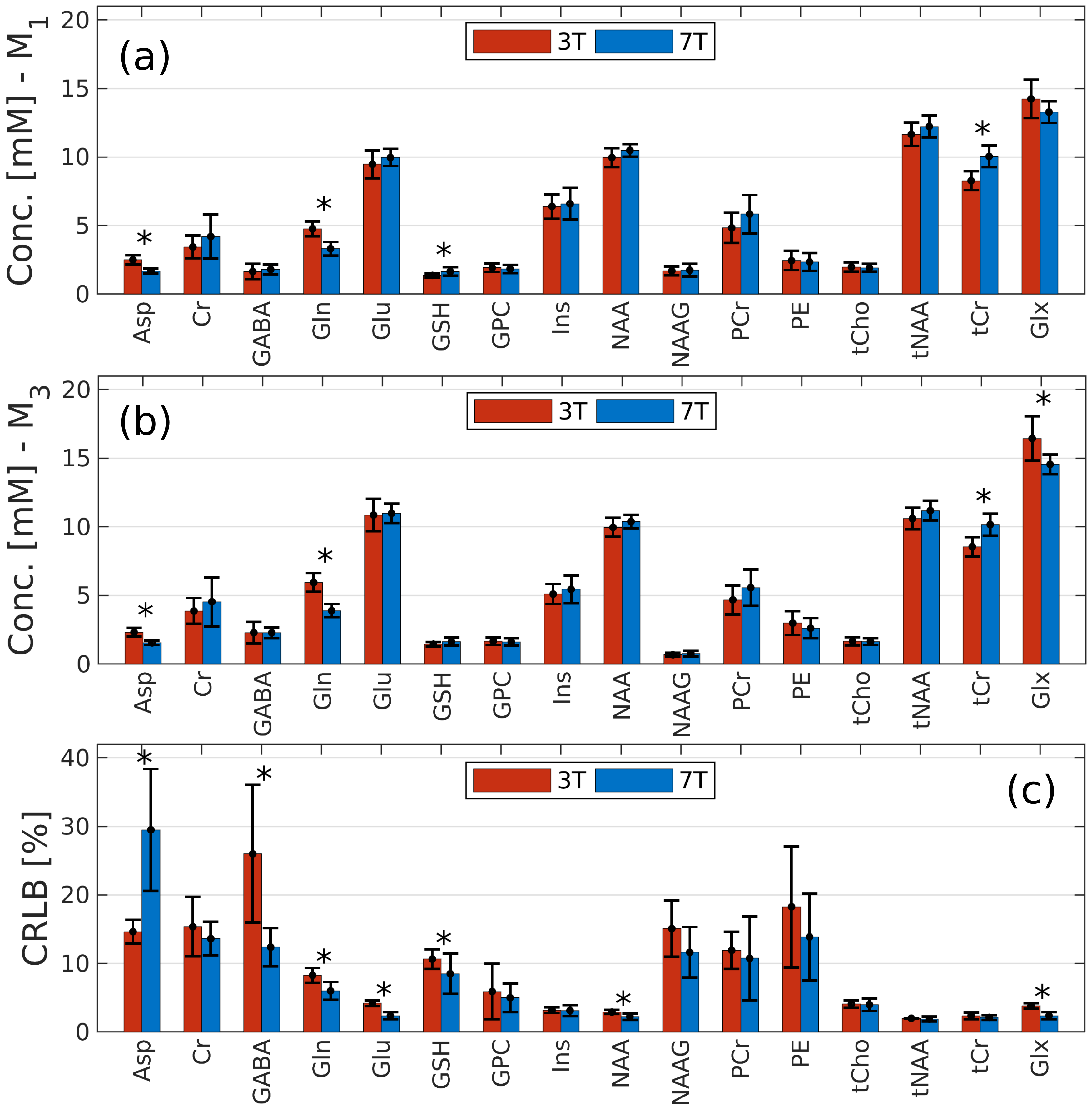
An example of the MRS voxel is shown in Figure 1 for 3T (a) and 7T (b). Figure 2 illustrates the spectra of a representative subject obtained with LCModel. A total of 12 metabolites were reliably measured following the aforementioned conditions. Figure 3 shows the metabolite concentrations plotted against φGM for selected metabolites. Figure 4 shows a comparison of M1 (a) and M3 (b) and the corresponding CRLB values (c). Concentrations of Asp, Gln, GSH, and tCr were significantly different between 3T and 7T. The concentrations of GSH that were initially significantly different (a) were insignificant when evaluated using M3 (b). For Glx, the concentrations that were initially insignificant when using M1 (a), became significant when using M3 (b).Discussion and Conclusions
We have shown the preliminary results of the performance of three methods applied for the quantification of the neurochemical profile of the striatum using single-voxel STEAM at 3T and 7T. We have provided a quantitative assessment of the concentration ratio for the striatum and the surrounding WM for 12 metabolites. We demonstrate that using the concentration ratio tends to give more accurate results compared to the case in which equal concentrations in GM and WM are assumed. Simulations considering the statistical significance using different tissue volume fractions and sequence timings are being performed.Acknowledgements
AG is half supported by the Shota Rustaveli National Science Foundation, Tbilisi, Georgia. Grant number JFZ_18_02. MS is supported by the Else Kröner-Fresenius-Stiftung (grant number 2019_EKES.02). We would like to acknowledge E.J. Auerbach and M. Marjanska (Center for Magnetic Resonance Research and Department of Radiology, University of Minnesota, USA) for the development of the STEAM and FASTESTMAP sequences for the Siemens platform, which was provided by the University of Minnesota under a C2P agreement. We thank Rick Claire for proofreading the abstract.
References
1. Gasparovic C, Song T, Devier D, et al. Use of tissue water as a concentration reference for proton spectroscopic imaging. Magn. Reson. Med. 2006;55(6):1219–1226.
2. Hetherington HP, Pan JW, Mason GF, et al. Quantitative 1H spectroscopic imaging of human brain at 4.1 T using image segmentation. Magn Reson Med. 1996;36(1):21-29.
3. Harris AD, Puts NA, Edden RA. Tissue correction for GABA-edited MRS: Considerations of voxel composition, tissue segmentation, and tissue relaxations [published correction appears in J Magn Reson Imaging. 2017;46(1):312]. J Magn Reson Imaging. 2015;42(5):1431-1440.
4. Tkac I, Starcuk Z, Choi IY, et al. In vivo 1H NMR spectroscopy of rat brain at 1 ms echo time. Magn Reson Med. 1999;41(4):649-656.
5. Marjańska M, McCarten JR, Hodges J, et al. Region-specific aging of the human brain as evidenced by neurochemical profiles measured noninvasively in the posterior cingulate cortex and the occipital lobe using 1H magnetic resonance spectroscopy at 7 T. Neurosci. 2017;354:168-177.
6. Giapitzakis IA, Shao T, Avdievich N, et al. Metabolite-cycled STEAM and semi-LASER localization for MR spectroscopy of the human brain at 9.4T. Magn Reson Med. 2018;79(4):1841-1850.
7. Brant-Zawadzki M, Gillan GD, Nitz WR. MP RAGE: a three-dimensional, T1-weighted, gradient-echo sequence - initial experience in the brain. Radiology. 1992;182(3):769-775.
8. Marques JP, Kober T, Krueger G, et al. MP2RAGE, a self bias-field corrected sequence for improved segmentation and T1-mapping at high field. Neuroimage. 2010;49(2):1271-81.
9. Gruetter R. Tkáč I. Field mapping without reference scan using asymmetric echo-planar techniques. Magn Reson Med. 2000;43(2):319-23.
10. Schär M, Vonken E. J, Stuber M. Simultaneous B0- and B1+-map acquisition for fast localized shim, frequency, and RF power determination in the heart at 3 T. Magnetic resonance in medicine. 2010;63(2): 419-426.
11. Simpson R, Devenyi GA, Jezzard P, et al. Processing and Simulation of MRS DataUsing the FID Appliance (FID-A)—An Open Source, MATLAB Based Toolkit. Magnetic Resonance in Medicine. 2017;77:23–33.
12. Soher B. J, Semanchuk P, Todd D, et al. VeSPA: Integrated applications for RF pulse design, spectral simulation and MRS data analysis. Proc. Intl. Soc. Mag. Reson. Med. 2011.
13. Henry PG, Marjanska M, Walls JD, et al. Proton‐observed carbon‐edited NMR spectroscopy in strongly coupled second‐order spin systems. Magn Reson Med. 2006;55(2):250‐257.
14. Govindaraju V, Young K, Maudsley AA. Proton NMR chemical shifts and coupling constants for brain metabolites. NMR Biomed. 2000;13(3):129‐153.
15. Kaiser LG, Marjanska M, Matson GB, et al. 1H MRS detection of glycine residue of reduced glutathione in vivo. J Magn Reson. 2010;202(2):259‐266.
16. Govind V, Young K, Maudsley AA. Corrigendum: proton NMR chemical shifts and coupling constants for brain metabolites. Govindaraju V, Young K, Maudsley AA, NMR Biomed. 2000;13:129–15. NMR Biomed. 2015;28(7):923‐924.
17. Tkáč I, Öz G, Adriany G, et al. In vivo 1H NMR spectroscopy of the human brain at high magnetic fields: metabolite quantification at 4T vs. 7T. Magn Reson Med. 2009;62(4):868-879.
18. Zhang Y, Brady M, Smith S. Segmentation of brain MR images through a hidden Markov random field model and the expectation-maximization algorithm. IEEE Trans Med Imaging. 2001;20(1):45-57.
19. Patenaude B, Smith SM, Kennedy DN, et al. A Bayesian model of shape and appearance for subcortical brain segmentation. Neuroimage. 2011;56(3):907-922.
20. Visser E, Keuken MC, Douaud G, et al. Automatic segmentation of the striatum and globus pallidus using MIST: Multimodal Image Segmentation Tool. Neuroimage. 2016;125:479-497.
21. Ethofer T, Mader I, Seeger U, et al. Comparison of longitudinal metabolite relaxation times in different regions of the human brain at 1.5 and 3 Tesla. Magn Reson Med. 2003;50(6):1296-1301.
22. Mlynárik V, Gruber S, Moser E. Proton T (1) and T (2) relaxation times of human brain metabolites at 3 Tesla. NMR Biomed. 2001;14(5):325-331.
23. Xin L, Schaller B, Mlynarik V, et al. Proton T1 relaxation times of metabolites in human occipital white and gray matter at 7 T. Magn. Reson. Med. 2013.
24. Marjańska M, Auerbach EJ, Valabrègue R, et al. Localized 1H NMR spectroscopy in different regions of human brain in vivo at 7 T: T2 relaxation times and concentrations of cerebral metabolites. NMR Biomed. 2012;25(2):332-339.
Figures