2019
Quantification of 2D-MRSI Datasets using Random Forest Regression Comparing to Prior Knowledge Based Spectral Fitting applied to Brain Tumors1Neuroradiology / Support Center for Advanced Neuroimaging (SCAN), University Hospital and Inselspital, University Bern, Bern, Switzerland, 2Neurosurgery, University Hospital and Inselspital, University Bern, Bern, Switzerland
Synopsis
Robust spectral quantification is essential in clinical 1H-MRSI. A machine-learning technique to quantify 2D-MRSI data aiming to mimic prior-knowledge fitting of the data of glioma patients at 3T. A Random-Forest Regression method was applied on MRSI-data aiming at obtaining improved starting values for the NLLS-algorithm. Enhanced starting values can bring significant developments in the spectral fit quality in clinical 1H-MRS. Different noise levels were compared in order to verify and improve the fitting. Results indicate that this novel approach could increase fitting precision and eliminate possible errors caused by the using uniform starting values and improve method for MRSI-data quantification.
Introduction
Proton MRS(I) is a technique that enables non-invasive characterization of normal and pathologic brain tissues on a metabolic level. Non-linear least squares (NLLS) fitting methods1-4 are used to quantify the detectable metabolites in these datasets. These NLLS-techniques will be regarded in this abstract as golden standard. Recently several artificial intelligence (AI) approaches have been proposed all aiming at performing spectral quantification using AI. Two different AI methods are described: (a.) machine learning (ML) methods like Random Forest regression5, and (b.) deep learning approaches 6,7. In this abstract we will describe the complete processing pipeline necessary to successfully apply and use Random Forest Regression8 applied to the fitting problem. The method presented here is similar to the ML-method presented in reference5. Here we studied semi-LASER based 1H-2D-MRSI datasets with application to primary brain tumors. Large portions of the described methodology were implemented in the native spectrIm plugin9 using quantification NLLS-TDFDFit method3. spectrIm is a plugin of jMRUI2.Method
Several RF-regressors were computed based on a pre-existing prior knowledge TDFDFit-fitting model which is part of the spectrIm-plugin of jMRUI. This prior-knowledge spectral modelling tool is displayed in Figure 1. It enables easy to define and use advanced prior-knowledge based modelling of which the prior-knowledge model is described in detail in reference9.The signal preparation, learning and prediction workflow is displayed in Figure 2. After the user has defined a prior knowledge model, the prior-knowledge model-parameters were subsequently randomly variated and time- and frequency-domain responses were computed that all satisfied the prior knowledge model conditions. These randomly varied model parameters together with the corresponding time domain and frequency domain signals are stored in a comma-separated values (csv) file which is used as input for the training RF-regressors, that on their turn are used as predictors of the model-parameters.
The random forest-based regressor was computed in Python using the sklearn library and it was trained on 10'000 cases, with an architecture in which n_estimator=270 and a maximum depth max_depth=17. The best n_estimator and max_depth parameters for the regressor were found by performing a nested cross validation each evaluating the estimator performance and error generalization of the underlying model and its hyperparameters. The data consisted of absorption and dispersion points in both frequency-domain (FD) and time-domain (TD), normalized by the first point in TD. The selection of the training dataset points was done by identifying those regions of interest in MRSI TD and FD-responses with maximal information content for the training. The chosen interval in FD were between 0.75ppm and 5.25ppm and in TD only the first 140 acquisition points of 1024 points of the FID was chosen. For several response noise levels separate RF-regressors were computed all satisfying the same prior knowledge model. For three selected noise levels, namely relative noise level 1 = 0.5, noise level 2 = 4; and noise level 3 = 8 result were obtained to predict an in vivo brain-tumor dataset. This approach enables the study of the influence of the noise level in the training data on the RF-regressor performance. Noise level 0.5 matches the noise level of the in vivo datasets best. It was hypothesized that this RF-regressor performs best. The RF-regressor will learn the relation between the common frequency shift, common Lorentzian common zero order phase and all area parameters of the model (total 10 parameters). The following metabolites were quantified: NAA, Cho, Cr, Lac, myo-inositol, and Glu. The obtained RF-regressors were then applied on the same TE semiLASER 2D-MRSI brain tumor data, to compare their performance on an in vivo case.
Results
Figure 3 shows the ground truth (GT) metabolite peak area maps of NAA, Cho, Cr, Glx of the prior-knowledge model, and the above mentioned predicted areas for 3 different noise levels. Figure 4 visualizes the correlation between the peak areas of GT and noise level 0.5 predictions for the metabolites. Finally Figure 5 shows examples of the training signals in TD and FD, and sample spectra of the GT and predicted spectra.Discussion and Conclusion
The maps of all prediction in Figure 3 nicely match the GT maps and the scatter plots between the GT and the 3 RF-regressors based on three different noise levels. For the optimal noise level equal to 0.5, Figure 4 shows the high level of correlation between all GT and metabolite area predictions. The variance in the plots are in the range that can be expected based on Cramér-Rao minimum variance bounds. This means that RF-regression could be used as direct quantification engine for this type of data, or predicted model parameters could be used as improved starting values for NLLS-fitting.Training RF-regressors on both TD- and FD-signals gave best result, while training on FD-only gave worse results that on training on TD-signals only. The RF-regressor for the lowest noise level 0.5 performed best.
Acknowledgements
This project has received funding from the European Union’s Horizon 2020 research and innovation programme under grant agreement No 813120.References
1. Provencher SW. Estimation of metabolite concentrations from localized in vivo proton NMR spectra. Magn Reson Med [Internet]. 1993 Dec 1 [cited 2020 Dec 14];30(6):672–9. Available from: https://onlinelibrary.wiley.com/doi/full/10.1002/mrm.1910300604
2. Stefan D, Cesare F Di, Andrasescu A, Popa E, Lazariev A, Vescovo E, et al. Quantitation of magnetic resonance spectroscopy signals: the jMRUI software package. Meas Sci Technol [Internet]. 2009 Oct 1 [cited 2019 Apr 8];20(10):104035. Available from: http://stacks.iop.org/0957-0233/20/i=10/a=104035?key=crossref.d6dc8615cb88426675ce9638bb30b723
3. Slotboom J, Boesch C, Kreis R. Versatile frequency domain fitting using time domain models and prior knowledge. Magn Reson Med [Internet]. 1998;39(6):899–911. Available from: http://www.ncbi.nlm.nih.gov/pubmed/9621913
4. Wilson M, Reynolds G, Kauppinen RA, Arvanitis TN, Peet AC. A constrained least-squares approach to the automated quantitation of in vivo (1)H magnetic resonance spectroscopy data. Magn Reson Med. 2010/09/30. 2011 Jan;65(1):1–12.
5. Das D, Coello E, Schulte RF, Menze BH. Quantification of metabolites in magnetic resonance spectroscopic imaging using machine learning. In: Lecture Notes in Computer Science (including subseries Lecture Notes in Artificial Intelligence and Lecture Notes in Bioinformatics) [Internet]. Springer Verlag; 2017 [cited 2020 Dec 14]. p. 462–70. Available from: http://link-springer-com-443.webvpn.fjmu.edu.cn/chapter/10.1007/978-3-319-66179-7_53
6. Ringer AJ, Guterman LR, Hopkins LN, Fleischmann A, Fandino J, Slotboom J, et al. Site-specific thromboembolism: a novel animal model for stroke. AJNR Am J Neuroradiol [Internet]. 2004 Feb 1 [cited 2017 Nov 21];25(2):329–32. Available from: http://www.ncbi.nlm.nih.gov/pubmed/14970041
7. Lee H, Lee HH, Kim H. Reconstruction of spectra from truncated free induction decays by deep learning in proton magnetic resonance spectroscopy. Magn Reson Med [Internet]. 2020 Aug 8 [cited 2020 Dec 14];84(2):559–68. Available from: https://onlinelibrary.wiley.com/doi/abs/10.1002/mrm.28164
8. Breiman L. Random forests. Mach Learn. 2001;45(1):5–32.
9. Pedrosa de Barros N, McKinley R, Knecht U, Wiest R, Slotboom J. Automatic quality control in clinical 1 H MRSI of brain cancer. NMR Biomed [Internet]. 2016 May [cited 2018 Jul 4];29(5):563–75. Available from: http://doi.wiley.com/10.1002/nbm.3470
10. Slotboom J, Brekenfeld C, Kiefer C, Kreis R, Remonda L, Schroth G. A Graphic Tool for Fast Interactive Spectroscopic Prior Knowledge Modeling and Prior Knowledge Database Management [Internet]. ISMRM. 1998 [cited 2020 Dec 14]. p. 2263–2263. Available from: https://www.researchgate.net/profile/Gerhard_Schroth2/publication/266881513
Figures
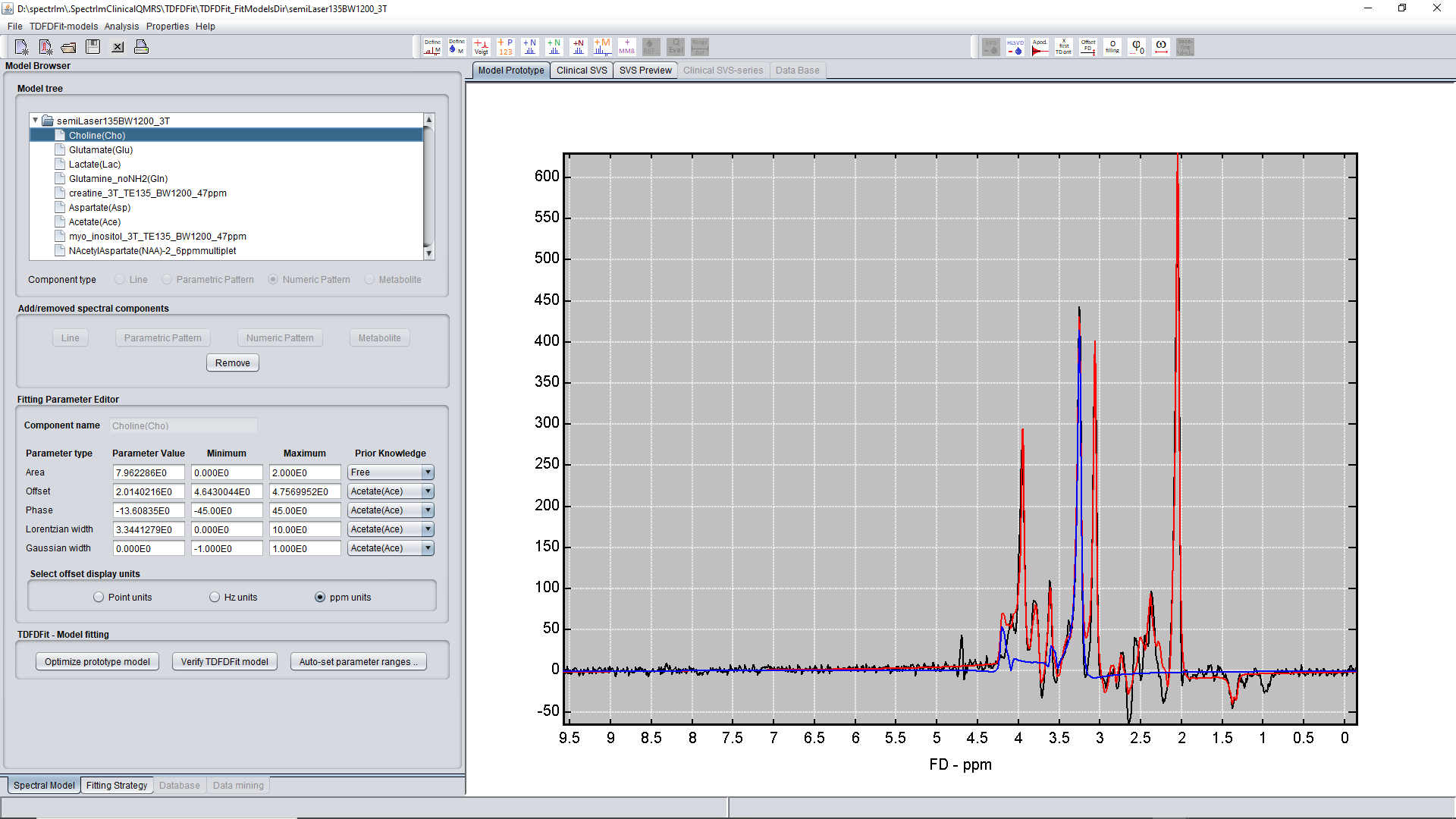
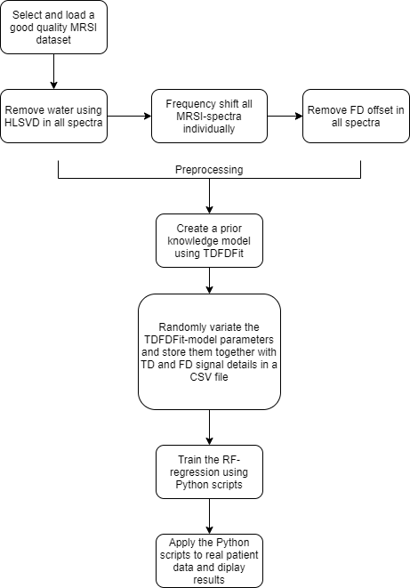
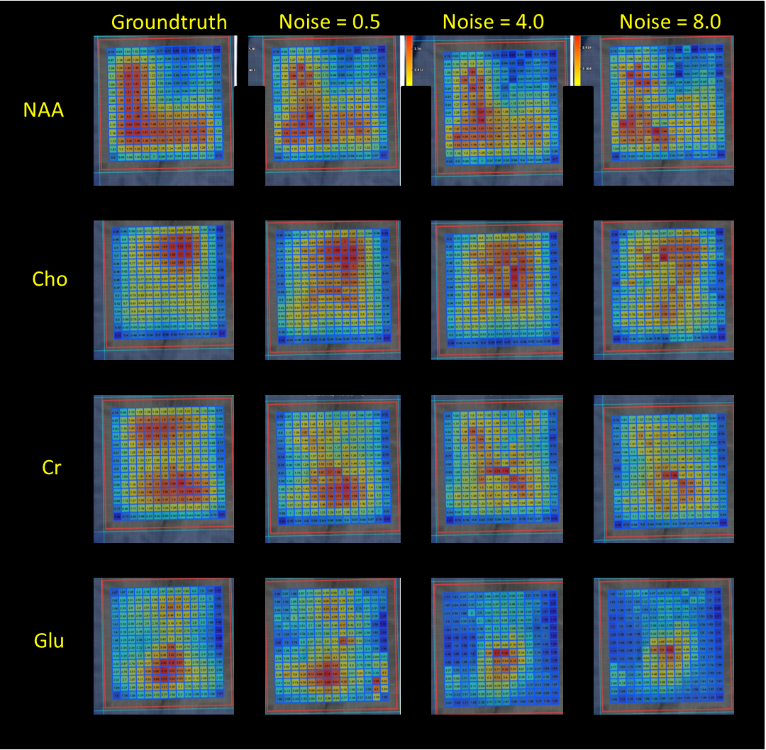
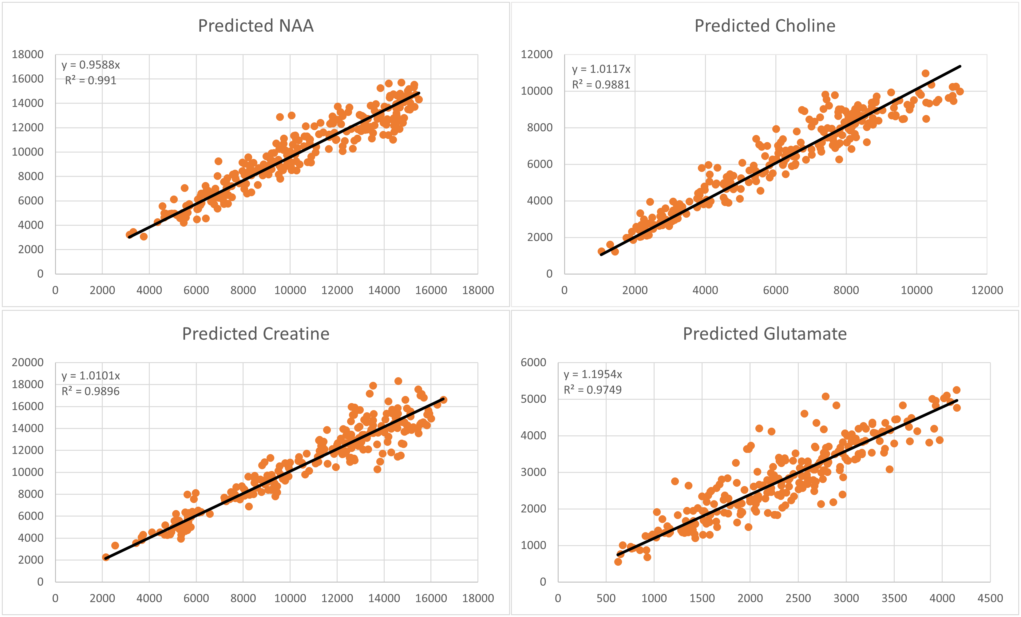
Figure 5:
A) shows an example of concatenation of the FD-absorption, FD-dispersion, TD-absorption and TD-dispersion signals used to train the noise-0.5 case.
B) same as A for noise-4 case
C) same as A for noise-4 case
D) in blue predicted spectrum in blue and GT in green for noise 0.5 regressor using complex TD response part only.
E) same as D) using complex FD part only.
F) same as D) but using RF-regressor based on noise = 8. Still very good prediction.
G) same as F) but using TD and FD based RF-regressor based on noise = 0.5; the best case.