Introduction

The current state of the art methodologies for metabolite quantification of in vivo MR spectroscopy uses nonlinear least-squares (NLLS) methods, which are very computational time consuming for a large number of spectra. For instance, in echo-planar spectroscopic imaging (EPSI), one dataset is recorded within 10-15 minutes of scanning time and can result in more than 100.000 spectra. For this reason, ultra-fast post-processing and quantification methods are required to make the EPSI technology attractive for clinical use. Recently, deep learning technologies have shown to be an extremely powerful tool for metabolite quantification of both simulated^1,2 and real³ spectra.
The aim is to achieve fast processing and quantification of MRSI-data on a time scale that is acceptable for daily clinical use. In this abstract we present and compare two different deep CNN architectures, aiming at performing prior knowledge metabolite quantification, and compare their performance to an NLLS-fitting algorithm (TDFDfit). We show the performance of the two algorithms in a set of 2 healthy persons as well as in a brain tumor patient.

Methods

Training dataset: We simulated a dataset of MRS spectra consisting of 9 different metabolites (Cho, Glu, Lac, Gln, Cre, Asp, Ace of NAA (further indicated as Ace), Myo Inositol, NAA-Asp). Each metabolite basis set was simulated using NMRScope-B, which is a plugin of jMRUI software. The training dataset (model parameters, time-domain (TD), and frequency domain (FD) responses) which obey prior knowledge model conditions were randomly generated within pre-sets of parameter ranges created using spectrIm, which is another jMRUI plugin. In this way, we obtained a set of 20.000 TD/FD responses with the corresponding set of model parameters consisting of nine areas (one for each metabolite), one common offset difference parameter, one common Lorentzian width difference parameter, and one common phase difference parameter. 80% of the data was dedicated to training and the remaining 20% was used for validation.

Clinical dataset: The data used to study the performance in real in-vivo spectra, was measured in a 3T using the semiLASER 2D-MRSI pulse sequence (TE=135ms;TR=1500ms;N=1024) . Only the FD-responses were used as input for the developed neural networks and a ppm range set to 5.7-0.6ppm was used. These CNNs were used to predict the metabolite area parameters and compared the results with those obtained by TDFDFit and is regarded as ground truth.

Pre-processing of data: For the in-vivo data, the pre-processing consisted of water removal through HLSVD method, and frequency domain offset correction. Both training and in-vivo datasets were normalized by the area under the spectra and smoothed using the Savitzky-Golay⁴ filter with a window size of 3.

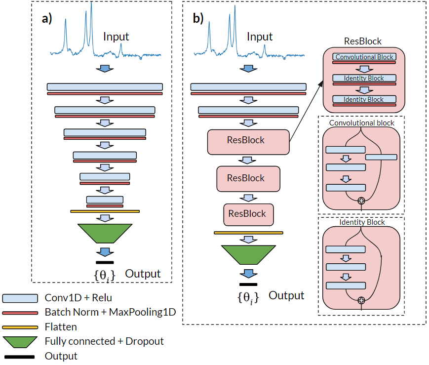
Neural Networks: We implemented two different neural networks, both based on the power of CNNs. The first development is a VGG-like⁵ architecture (from now on, called CNN) shown in Figure 1-a and the second is a ResNet-like network⁶, the latest was implemented with intermediates max pooling to avoid overfitting due to the big number of parameters. This ResNet is shown in Figure 1-b. ResNet has outperformed in a wide range of problems.
In both networks the training hyper-parameters we used were: mean squared difference as loss function, Adam as an optimizer, learning rate of 0.001, drop out with a rate of 0,1 and we set the maximum of epochs to be 100.

Results

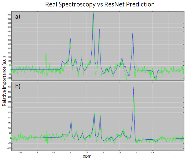
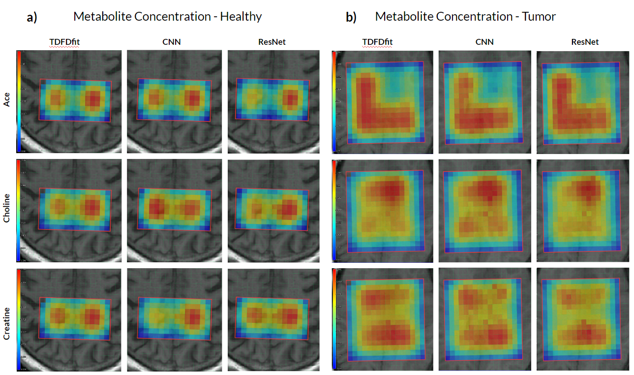
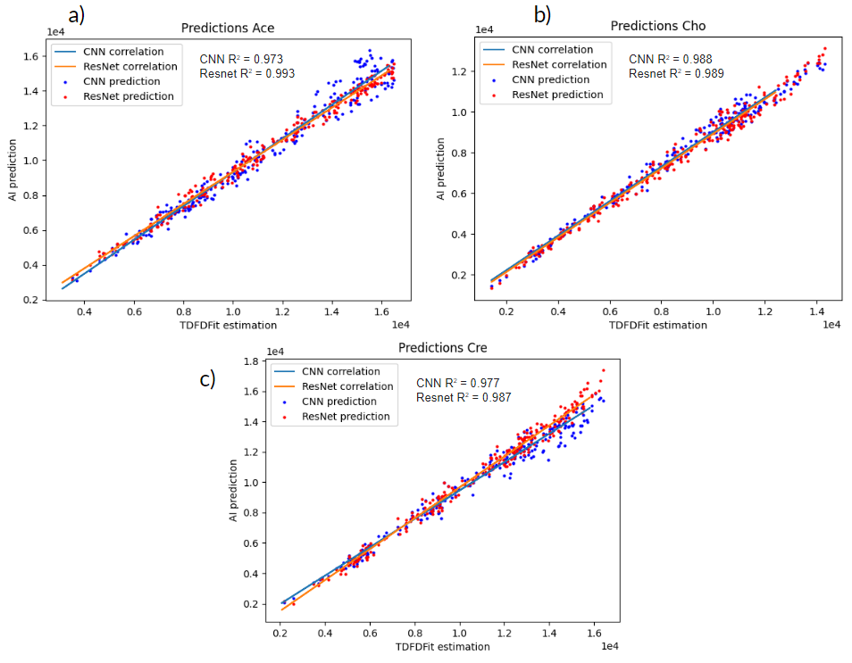
We analyzed the performance of the implemented networks on real patient data as described above. Figure 2 shows a comparison between the in vivo spectra and the ResNet predicted spectra for tumor spectrum (Figure 2.a) as well as for healthy brain tissue (Figure 2.b).
To visualize the performance for in vivo spectra, we generated metabolite maps of Cho, Cr, and Ace as shown in Figure 3. It is justified to conclude that ResNet has a better prediction of spatial metabolite distributions than CNN when compared to TDFDFit. We also found that the correlation between the predicted metabolites and the TDFDFit ground-truth is bigger for the ResNet than the CNN, as shown in Figure 4. However, ResNet consistently predicts a smaller area parameter for Ace, while CNN has a bigger variance but a slope that is closer to 1.
We applied the same analysis to two healthy patients and found the same behavior, even though the ResNet is more precise both methods reach an average difference up to 25% relative to TDFDFit.

Discusion

We observed that both neural network methods are suitable to find the correct spatial distribution of the metabolites being the ResNet more precise.
For in-vivo data, we found that both methods differ from the ground truth consistently by the same factor along with the metabolite areas, this could be induced by the smoothing pre-processing applied on the training and testing datasets. This could explain also why the healthy tissue, whit very narrows peaks compared with the tumor tissue, underperformed.

Acknowledgements

This project has received funding from the European Union’s Horizon 2020 research and innovation programme under grant agreement No 813120.