Introduction

Magnetic resonance spectroscopic imaging (MRSI) is a noninvasive tool for assessing brain metabolites and has been applied to patients with brain tumors, multiple sclerosis, epilepsy and psychiatric disorders. The accuracy of assessing brain metabolite levels highly relies on spectra quality. Artifacts, such as field inhomogeneity, insufficient lipid suppression and spurious peaks, could interfere spectra and make the interpretation challenging. The confirmation of spectral artifacts conventionally requires manual review by MRS experts. However, due to the large number of voxels from one 3D MRSI data, this step could be time-consuming. Several recent studies have reported machine learning models are able to filter voxels with artifacts automatically^1-5. One of these studies developed a convolutional neural network (CNN) model on 3T MRSI from patients with glioma and achieved an area under the curve (AUC) of 0.955. In this study, we evaluated the performance of this model on 7T MRSI data that were obtained from patients with different types of neurological diseases and examined features that could be included to improve its performance.

Methods

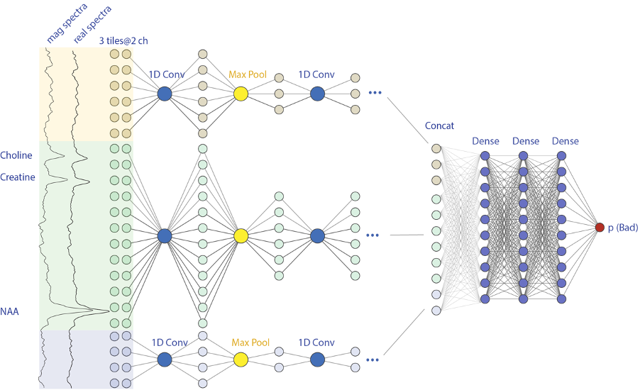
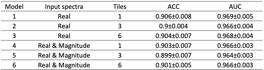
All MR data were performed using a 32-channel receive-only array with a volume transmit head coil on a GE 7T MR950 scanner. 3D MRSI data were obtained using spin-echo localization, TE/TR = 20/2000 ms, matrix size = 16-20x22x8 and nominal spatial resolution = 1cm3 and processed as described previously⁶. A total of 40 short MRSI datasets from 10 healthy controls, 10 patients with major depressive disorder, 10 patients with multiple sclerosis, and 10 patients with Parkinson’s Disease. In order to balance class portions, data with subject movement were included by purpose. Voxels outside brain mask or suppressed by outer volume suppression bands were excluded. Spectra with wide spectral linewidth (FWHM>0.10ppm) and/or large Cramer-Rao lower bounds (Cr CRLB>10) were labelled as “bad”. The remaining were manually examined by an expert and labeled as “bad” or “good”. The final data consisted of 7,940/8,823 spectra labeled with “good/bad” and were randomly split into 8:1:1 for training, validation and testing. Additionally, segmentation of the brain was performed on T1 images with Harvard-Oxford subcortical structural atlases to get tissue ratios of cortical, subcortical, white matter, and cerebrospinal fluid. Spectra between 1.4ppm and 4.1 ppm were first standardized using sklearn.preprocessing.StandardScaler. Three types of inputs for spectra data were tested, including real spectra only, real concatenated imaginary spectra, and real concatenated magnitude spectra. Each spectrum was divided into 1, 3 or 6 tiles. Another optional input choice was to include tissue components as four individual channels. Each tile independently went through 6 convolutional and max pooling layers for feature extraction. After flattening, features from different tiles were concatenated and fed through two fully connected layers of 128 nodes then generated a scalar probability value (Figure 1). Models with different inputs and tiles were listed in Table 1. Each model was re-tested for 10 times and average accuracy (ACC) and AUC values were calculated. The pipeline was implemented in Python3 using Numpy, Pandas, Scikit-learn, and Tensorflow2 libraries.

Results and Discussions

In the study, we include datasets from healthy controls and patients with neurologic and psychiatric diseases, who had different type of metabolism. The performance of each model is illustrated in Figure 2. Our results showed adding atlas tissue information into the model did not improve the performance. There was no significant difference between different combinations of input. All models yielded similar performance at an ACC of 0.90 and AUC of 0.96-0.97, which indicated the generalizability of model for evaluating 7T MRSI data. However, several factors could limit our finding, such as the bias of one rater and two classifiers for spectral quality. Future work will include more raters for defining ground truth, evaluate inter-rater agreement, and implement Integrity Gradients⁷ methods to evaluate the features importance of trained models.

Acknowledgements

NIH R21HD092660